Minimizing remote storage usage and synchronization time using deduplication and multichunking: Syncany as an example
This post introduces my Master’s thesis “Minimizing remote storage usage and synchronization time using deduplication and multichunking: Syncany as an example”. I submitted the thesis in January 2012, and now found a little time to post it here.
The key goal of this thesis was to determine the suitability of deduplication for end-user applications – particularly for my synchronization application Syncany. As part of this work, the thesis introduces Syncany, a file synchronizer designed with security and provider independence as a core part of its architecture.
Contents
- Introduction
- Related Work
- Deduplication
- Syncany
- Implications of the Architecture
- Experiments
- Future Research
- Conclusion
- A. List of Configurations
- B. Pre-Study Folder Statistics
- C. List of Variables Recorded
- D. Best Algorithms by Deduplication Ratio
- E. Best Algorithms by Duration
- F. Best Algorithms by CPU Usage
- Bibliography
Download as PDF: This article is a web version of my Master’s thesis. Feel free to download the original PDF version.
1. Introduction
The recently arisen cloud computing paradigm has significantly influenced the way how people think of IT resources. Being able to rent computing time or storage from large providers such as Amazon or Rackspace has enabled a more flexible and cost-effective use of resources. While corporations mostly benefit from the significant cost savings of the pay-per-use model, private individuals rather use it as cheap external storage for backups or to share the private photo collection. Cloud-based backup and file sharing services such as Box.net, Dropbox or Jungle Disk have become very popular and easy-to-use tools for exactly this purpose. They deliver a very simple and intuitive interface on top of the remote storage provided by storage service providers. Key functionalities typically include file and folder synchronization between different computers, sharing folders with other users, file versioning as well as automated backups.
While their feature set and simplicity are very appealing to users, they all share the property of being completely dependent of the service provider – especially in terms of availability and confidentiality. This highlights the importance of the providers and outlines their central role in this scenario: Not only do they have absolute control over the users’ data, they also have to make sure unauthorized users cannot access it. While many users have been willing to trade this lack of confidentiality for a more convenient user experience, this level of trust towards the provider disappears when the data is very private or business critical.
To address the issues outlined above, this thesis introduces Syncany, a file synchronization software that allows users to backup and share certain files and folders among different workstations. Unlike other synchronization software, Syncany is designed with security and provider independence as an essential part of its architecture. It combines high security standards with the functionalities and ease of use of a cloud-based file synchronization application. In particular, Syncany does not allow access to data by any third party and thereby leaves complete control to the owner of the data. The goal of the architecture is to provide the same functionality as existing solutions, but remove provider dependencies and security concerns.
In contrast to other synchronization software, Syncany offers the following additional functionalities:
Client-side encryption: Syncany encrypts files locally, so that even untrusted online storage can be used to store sensitive data.
Storage abstraction: Syncany uses a plug-in based storage system. It can be used with any type of remote storage, e.g. FTP, Amazon S3 or WebDAV.
Versioning: Syncany stores the entire history of files and folders. Old revisions of a file can be reconstructed from the remote storage.
Even though these features are not new ideas on their own, their combination is a rather new approach and does, to the best of the author’s knowledge, not exist in other file synchronization applications.
1.1. Problem Description
While Syncany is very similar to other file synchronizers from an end-user’s point of view, its functionalities demand for a more complex architecture. Especially when looking at the storage abstraction and versioning requirements, traditional synchronization software or frameworks cannot be used. Synchronizers such as rsync or Unison, for instance, completely lack any kind of versioning functionalities. Version control systems such as Git or Subversion on the other hand only support a few storage types and entirely lack encryption.
A rather naive approach to create a file synchronizer with the desired functionalities is to simply encrypt all files locally and then transfer them to the remote storage using the respective transfer protocol. Once a file is changed locally, it is copied using the same protocol. To ensure that the old version of the file is still available, new revisions are copied to a new filename.
While this approach is very simple and can be easily implemented using any kind of storage, it has many obvious flaws. Among others, it always copies files as a whole even if only a few bytes have changed. Because of that, the amount of data stored on the remote storage increases very quickly. Consequently, uploading updates and reconstructing files from the remote storage takes significantly longer than if only changes were transferred.
Syncany overcomes this problem with its own architecture: Storage abstraction, versioning and encryption are part of the core system. Using deduplication technology, Syncany delivers the same features as other synchronizers, and minimizes its storage requirements at the same time. Especially in terms of storage reduction, deduplication has proven to be very effective in various hardware and software based backup systems. In end-user applications, however, the technology is rarely used to its full extent.
Certainly one of the reasons for that is that the algorithms used in deduplication systems are very CPU intensive. The underlying data is analyzed very thoroughly and frequent index lookups increase the CPU usage even further. In most cases, only very coarse-grained deduplication mechanisms are used on the client and further data-reducing algorithms are performed on the server.
Another issue is created when combining deduplication with the storage abstraction concept. Due to the fact that deduplication algorithms generally create a large number of small files, the upload and download time tends to be very high. For Syncany, that means a high synchronization time between participating clients.
Overall, using the concept of deduplication as part of Syncany’s core is both the solution and the problem. On the one hand, it is one of the key technologies to create a functioning file synchronizer. Among others, it enables versioning, minimizes disk usage on the remote storage and reduces the amount of transferred data. On the other hand, the technology itself causes problems on the client. Examples include high CPU usage and an increased amount of upload and download requests.
1.2. Goal
Having seen a variety of issues in the overall architecture, this thesis focuses on very few of these aspects. In particular, the goal is to solve the problems created by introducing deduplication as a core concept. In the scope of this thesis that means demonstrating that deduplication is a valid technology for an end-user application and tackling the issues it raises. The overall goal is to find the deduplication algorithm best suited for Syncany’s environment as well as to make sure that synchronization time between clients is minimal.
Broken down into individual parts, the thesis aims to fulfill the following goals:
Find a suitable deduplication algorithm for Syncany: Since deduplication is mostly used on dedicated server machines, the requirements for client machines differ from the usual environment. An algorithm is suitable for Syncany if it minimizes the amount of data that needs to be stored, but at the same time makes sure that the client resources are not too excessively used and synchronization time is adequate.
Minimize the synchronization time between Syncany clients: The synchronization time is the sum of all subsequent processes performed to synchronize two or more Syncany clients. Minimizing it means accelerating the deduplication algorithm on the one hand, but also reducing the transfer time to and from the remote storage.
In order to fulfill these goals, this thesis analyzes the implications of the Syncany architecture on potential algorithms and performs experiments to find the optimal deduplication algorithm. It furthermore introduces the multichunk concept, a technique to reduce the upload and download time to and from the remote storage and validates its efficiency in experiments.
1.3. Structure
After this brief introduction, chapter 2 introduces related research and technologies. It particularly talks about research that influenced the development of Syncany. Among others, it discusses file sychronizers such as rsync and Unison in the context of the remote file synchronization problem. It then briefly presents the concepts of version control systems and finally explains the basic idea of distributed file systems.
Chapter 3 presents the fundamentals of deduplication. It gives a short overview of the basic concept and distinguishes deduplication from other capacity reducing technologies such as compression. The chapter then introduces relevant hardware and software based deduplication systems and briefly elaborates on their respective properties. Subsequently, it explains the different types of chunking methods – namely whole file chunking, fixed-size chunking, variable-size chunking and file type aware chunking. Finally, the chapter introduces and explains different quality measures for comparing deduplication mechanisms against each other.
After focusing on the technologies used, chapter 4 presents Syncany and explains how deduplication is used in it. It furthermore explains the motivation behind the software, defines high level requirements and elaborates on design choices made in the development. It then briefly introduces Syncany’s architecture and the concepts used in the software.
Chapter 5 illustrates the implications of the architecture on the thesis’ goals. Among others, it elaborates on bandwidth and latency issues and introduces the multichunk concept. It then discusses the design of potential deduplication algorithms and chooses the algorithm parameters for the experiments.
Chapter 6 uses these parameters to perform three experiments on different datasets. Experiment 1 aims to find the best parameter configurations with regard to chunking efficiency. Experiment 2 tries to maximize the upload bandwidth and experiment 3 measures the reconstruction time and size.
Before concluding the thesis, chapter 7 briefly discusses possible future research topics.
Download as PDF: This article is a web version of my Master’s thesis. Feel free to download the original PDF version.
2. Related Work
This thesis describes a synchronization software as well as a deduplication based algorithm. It uses techniques known in various disciplines and systems. This chapter introduces related research and projects from the areas of synchronization, version control and distributed file systems.
2.1. Synchronization Software
Synchronization software attempts to efficiently solve the remote file synchronization problem [44,46,47,49], i.e. the problem of keeping several replicas of a file or folder up-to-date throughout different locations. Since the problem occurs frequently in many different settings and applications, it is the goal of several algorithms and projects to solve it in an efficient manner with regard to their particular application. While the goal is the same (or at least very similar) in all cases, the solutions differ fundamentally due to the application’s requirements.
Depending on the main purpose of the software, algorithms either focus on constantly updating other replicas or on populating updates only periodically. Since in many situations hourly or even daily updates are sufficient, most synchronization and backup software follow the latter paradigm [44,50]. Another way of differentiating existing algorithms is to divide them into single-round and multi-round protocols. While multi-round algorithms often use recursive divide-and-conquer mechanisms on a hash-basis to detect changes in remote files, single-round protocols mostly use non-recursive fixed-size or variable-size chunking mechanisms to compare file contents [48,51].
A very widely used synchronization software is the open source tool rsync [44]. It is based on the rsync algorithm which uses a fixed-size single round synchronization protocol. rsync creates file and block lists of both local and remote file system, compares them and transfers the changed blocks in a single batch per direction. While rsync efficiently groups changed blocks and compresses the stream to additionally accelerate the transfer, it requires both sides to actively gather file lists and generate checksums for each round it is run. This characteristic makes it unsuitable for frequent small changes on a big file base. Since it requires a server with rsync installed, it cannot be used with arbitrary storage.
A few research papers have attempted to improve the original single-round rsync design in terms of bandwidth savings for specific applications or even suggested new algorithms. Irmak et al. [48] use several techniques to optimize rsync’s single-round algorithm. In their approach they simulate a complete multi-round algorithm by using erasure codes for the computed hashes in each round. Other researchers have proposed multi-round algorithms [72,47,74] that use the advantages of the divide-and-conquer paradigm when comparing remote and local files. While these algorithms can perform better in terms of bandwidth [51], this advantage might be lost in wide area networks due to higher latencies [73].
Another well-known file synchronizer is Unison [50,56,57]. Similarly to rsync, it generates file lists of both sides, compares and then reconciles them. While rsync only synchronizes in one direction, Unison has a bi-directional synchronization algorithm. It divides the process of synchronization in the two phases update detection and reconciliation. In the first phase, it detects updates on both sides based on modification time and inode numbers. It marks files dirty if either one of these properties has changed with regard to the last synchronization run. In the second phase, it applies the updates based on a well-defined recursive multi-round synchronization algorithm.
Similar to rsync, Unison relies on a rolling checksum algorithm to detect the parts of a file that have changed. It only works with two replicas and strongly relies on the Unison software to be present on both sides. It hence shares rsync’s drawbacks regarding frequent updates of small files. However, since updates are detected using metadata rather than checksums, the Unison update detection phase is typically much shorter.
Traditional backup and synchronization software such as Unison and rsync concentrate on providing on-demand file synchronization. They are mostly used for synchronizing two replicas periodically or to backup files and folders overnight. For cases in which more frequent (near-live/real-time) updates are desired, they are mostly not suitable due to the significant overhead required for the generation of file lists.
For this use case, synchronizers such as iFolder (was at ifolder.com, site now defunct, July 2019), Dropbox or Jungle Disk offer a solution. Instead of only analyzing the files on-demand, they register watch listeners in the operating system and react whenever a file is changed locally. Since every file update is registered by the software, generating file lists is superfluous. Moreover, it allows for the automatic recording of file versions by the software.
Due to its simplicity, especially Dropbox has become very popular. It offers live synchronization or continuous reconciliation [57] on different operating systems and integrates in the native file manager. While its core functionality is synchronization, it additionally provides basic revision control features and simple Web hosting functionalities. Dropbox uses an rsync-like chunking algorithm and only transfers binary diffs of updated files to save bandwidth and remote storage. On the server side, Dropbox uses deduplication among all Dropbox users and stores encrypted file chunks on Amazon S3. 1
2.2. Version Control Systems
Similar to regular synchronization software, Version Control Systems (VCS) are designed to coordinate and synchronize files among different locations. However, while file synchronization and version control are closely related in terms of functionality, they are often used for entirely different purposes. The aim of synchronization algorithms is to identify the differences among two or more replicas in order to keep them up-to-date. Version control, however, does not only seek to synchronize the end state of two replicas, but the entire version history of each individual file. While VCS are best suitable for text files (e.g. source code), synchronization software is designed for arbitrary data. Even though VCS can handle binary files, their main focus lies on source control [3].
Unlike synchronization software, VCS keep track of changes made on a file, allow branching/forking file sets and can merge different branches into one. They keep track of updates using revision numbers and allow restoring older versions if necessary.
Widely used versioning software include the Concurrent Versions System (CVS), Apache Subversion (SVN) as well as the newer distributed revision control systems Git or Bazaar.
While their specific architecture differs in file formats and network protocols, they all rely on similar concepts. To store the contents of a revision, most of them record incremental changes of files and compare them to a snapshot of the same file. When a file is updated or restored, these changes are then sequentially applied to the snapshot [2,52]. While this is beneficial if the local and the remote file are only a few updates apart, it has a negative impact on performance and bandwidth if many updates have to be applied. Some revision control systems such as Mercurial counteract this behavior by creating more full snapshots so that the reconstruction mechanism can use closer snapshots and has to apply fewer deltas. Even though this benefits the overall update speed and improves the bandwidth, it adds significant storage overhead to the repository. Using this technique, the repository does not only save the changes of files, but also full copies of selected versions as snapshots.
While most versioning systems support multiple types of network protocols and sometimes even allow the use of arbitrary protocols, they are typically used with the respective standard protocol. Commonly supported are SSH/SFTP or HTTP/WebDAV.
To the best of the author’s knowledge, none of the widely used revision control systems support client-side encryption.
2.3. Distributed File Systems
Distributed file systems (DFS) such as the Network File System or the Andrew File System aim to transparently deliver storage services to clients. While they internally have to deal with similar problems as version control systems and synchronization software, their front-end is invisible to end-users. Distributed file systems are mounted on the operating system level (or as user file systems) and behave like local file systems. They are usually not visible to users and whenever a file is saved, changes are immediately applied to the attached replicas. Among others, they differ from VCS and synchronization software in the following aspects [50,56,57]:
The main purpose of distributed file systems is to be able to share files among different workstations and to extend the local disk space with remote storage. Unlike version control systems and file synchronizers, DFS do not keep a working copy on the local machine, but retrieve the file when it is opened by the user.
While most VCS and file synchronizers need an explicit user-originated commit command, DFS are usually based on implicit commits. That is they either block until the reconciliation operation is complete or they cache the files locally and publish the changes to the connected replicas at a later point in time. While nearly all distributed file systems today have a local cache, many operations are still synchronous and can negatively affect user experience [58].
A largely popular distributed file system is the Network File System (NFS). Originally designed in 1989 by Sun Microsystems [75], it is now the de-facto standard of the network file systems on Unix/Linux platforms. NFS exports parts of the server’s file system to its clients and interacts via lightweight Remote Procedure Calls (RPC). NFS clients do not have any permanent local caches and store metadata (such as file permissions) only for a very short time. In versions 2 and 3, the NFS protocol is entirely stateless and based around synchronous procedures, i.e. the server does not need to maintain any protocol state and RPCs block until the operation is complete. Since version 4 [76], NFS partially supports asynchronous calls and has improved caching performance. While NFS also works over wide area networks, its design specification focuses on local area networks with high bandwidth. Even though NFS reads and writes files in blocks, it does not use any bandwidth optimizing techniques and hence scales poorly [60].
The Low Bandwidth File System (LBFS) [36,38], developed at the University of Texas in Austin, addresses this problem by exploiting similarities among files and transferring only the altered file parts. LBFS maintains large caches on the local clients and performs most read and write operations on the local system. To minimize the bandwidth usage, it breaks files into chunks using the Rabin fingerprinting method and only transfers missing chunks to the LBFS server component. The original LBFS design extends the NFSv3 protocol with numerous performance related features [36]: (1) The local cache allows the client to operate mostly offline, (2) remote procedure calls are pipelined asynchronously and (3) traffic is compressed using Gzip. A slim lined version of LBFS [38] suggests further ways to minimize bandwidth consumption using the Pretty Light And Intuitive (PLAIN) fingerprinting algorithm. Rabin and PLAIN are further explained in chapter 3.4.3.
While NFS assumes a high bandwidth in the network, LBFS uses deduplication techniques to optimize bandwidth usage. However, even though LBFS outperforms NFS with small files, its file open latency for bigger files still relies on the network speed. Since LBFS only caches files after they have been opened before, file open operations can cause applications to freeze until the entire file is retrieved [38].
- 1 Since Dropbox is closed-source, the information in this paragraph cannot be verified with the source code. It is gathered from (a) the Dropbox Web site and help pages, (b) trusted Internet resources such as Dropbox employees, as well as (c)
straceoutput of the Dropbox binary on Linux.
Download as PDF: This article is a web version of my Master’s thesis. Feel free to download the original PDF version.
3. Deduplication
Since the core algorithms of Syncany strongly rely on deduplication, this chapter introduces the fundamental concepts known in this research area. The first part defines the term and compares the technique to other storage reducing mechanisms. The subsequent sections introduce different deduplication types and elaborate on how success is measured.
3.1. Overview
Data deduplication is a method for maximizing the utility of a given amount of storage. Deduplication exploits the similarities among different files to save disk space. It identifies duplicate sequences of bytes (chunks) and only stores one copy of that sequence. If a chunk appears again in the same file (or in another file of the same file set), deduplication only stores a reference to this chunk instead of its actual contents. Depending on the amount and type of input data, this technique can significantly reduce the total amount of required storage [41,42,45].
For example: A company backs up one 50 GB hard disk per workstation for all of its 30 employees each week. Using traditional backup software, each workstation either performs a full backup or an incremental backup to the company’s shared network storage (or to backup tapes). Assuming a full backup for the first run and 1 GB incremental backups for each workstation per week, the totally used storage after a three months period is 1,830 GB of data.1 Using deduplication before storing the backups to the network location, the company could reduce the required storage significantly. If the same operating system and applications are used on all machines, there is a good chance that large parts of all machines consist of the same files. Assuming that 70% of the data are equal in the first run and 10% of the 1 GB incremental data is identical among all workstations, the totally required storage after three months is about 510 GB. 2
While this is just an example, it shows the order of magnitude in which deduplication techniques can reduce the required disk space over time. The apparent advantage of deduplication is the ability to minimize storage costs by storing more data on the target disks than would be possible without it. Consequently, deduplication lowers the overall costs for storage and energy due to its better input/output ratio. Unlike traditional backups, it only transfers new file chunks to the storage location and thereby also reduces the bandwidth consumption significantly. This is particularly important if the user upload bandwidth is limited or the number of backup clients is very high.
Another often mentioned advantage is the improved ability to recover individual files or even the entire state of a machine at a certain point in time. In tape based backups, the restore mechanism is very complex, because the backup tape needs to be physically rewound to get the desired files. Using incremental backups on regular hard disks, the files of a given point in time may be split among different increments and hence needs to be gathered from various archives to be restored. In contrast, the restore mechanism in deduplication systems is rather simple. The index provides a file and chunk list for each backup, so restoring a file set is simply a matter of retrieving all chunks and assembling them in the right order.
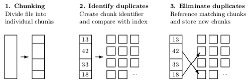 |
| Figure 3.1: Generic deduplication process (according to [35]). |
Figure 3.1 illustrates the generic deduplication process in three simple steps. In step 1, a file is broken into individual chunks. This can be done using fixed-size steps or variable-size chunking methods. In step 2, each of these chunks is then hashed to create a unique chunk identifier using a checksum algorithm such as MD5 or SHA-1. These identifiers are then looked up in the chunk index – a database that stores chunk identifiers and their mapping to the individual files. In step 3, chunks that already exist in the index are referenced to the current file and new chunks are added to the index.
3.2. Distinction and Characteristics
Similar to compression, deduplication encodes data to minimize disk usage. However, while compression is typically local to a file set or tree, deduplication is not bound to the location of a file on a disk or the date and time it is indexed. Compression mechanisms such as Lempel-Ziv (LZ) or Deflate have no persistent dictionary or index outside the created archive file. Once the compression algorithm is terminated, the index is written to the archive file and then purged from the memory. In contrast, deduplication follows a more stateful approach. Every chunk that a deduplication algorithm encounters is looked up in a global chunk index which is kept in the operating system’s memory or in a database. Depending on the use case, this index might even be distributed among different computers.
Unlike compression algorithms, deduplication does not describe exact algorithms to encode data in a certain way. Instead, it rather describes the general mechanisms, processes and design considerations. Deduplication does not have any standardized widely spread algorithms (such as LZ77 or PKZIP in data compression), but rather points out where, when and how it occurs. This particularly includes the following aspects [40,35]:
Location: Deduplication can be performed at different locations. Depending on the participating machines and steps in the customized deduplication process, it is either performed on the client machine (source-side) or near the final data store (target-side). In the former case, duplicates are removed before the data is transmitted to its storage. Since that conserves network bandwidth, this option is particularly useful for clients with limited upload bandwidth. However, since deduplication needs to analyze each file very closely, it can significantly increase the load on the client CPU. In the latter case, the chunking and indexing is done on the server and hence does not consume processing time on the client, but on the server machine. Since this method potentially transfers duplicate data, it is only acceptable if the client’s upload bandwidth is sufficient.
Time: Depending on the use case, deduplication is either performed as the data is transferred from the source to the target (in-band or in-line) or asynchronously in well-defined intervals (out-of-band or post-process). In the former case, data written to the target storage does not contain any duplicate chunks. Duplicates are identified and eliminated on the client or server as part of the data stream from source to target. In out-of-band deduplication systems on the other hand, the original data is written to the server storage and only later cleaned from duplicates. The in-band approach requires no post-processing and minimizes the required storage immediately. However, depending on the amount of data, this approach can cause a bottleneck in terms of throughput on the server side. Even though the out-of-band approach solves the bottleneck problem, it needs to buffer the undeduplicated data for the time between the deduplication runs. That is the server potentially needs multiple times the amount of disk space just so it can retain duplicate data.
Chunking method: Deduplication breaks files into small chunks in order to detect duplicates. The method used for chunking largely influences the deduplication success and can also affect the user experience. Literature differentiates four distinct cases [35,42,43,61]: Whole file chunking treats entire files as chunks (independent of their size), fixed-size chunking defines chunk boundaries by fixed offsets, variable-size chunking uses fingerprinting algorithms to determine the chunk boundaries and format-aware chunking (or file type aware chunking) handles files differently according to their file type. Details on these methods are discussed in section 3.4.
Identifying duplicate chunks: To save storage space, deduplication references redundant data instead of copying its contents. This concept relies on the assumption that each individual chunk has its own identity, i.e. an identifier by which it can be unambiguously referenced. For each chunk of a file, this identifier is calculated and compared to the global chunk index. If a chunk with a matching identifier is found in the database, the two chunks are assumed to be identical and the existing chunk is referenced. If not, the new chunk is added to the index. That is if two chunk identifiers are identical, the contents of the two chunks are also assumed to be identical. Depending on the number space of the chunk identifiers, this assumption can more or less likely lead to false matches and hence to data corruption.
False matches: Since the identifier is a representation of the chunk contents, deduplication systems typically use cryptographic hash functions such as MD5 or SHA-1 to calculate the chunk identity [8]. Even though hash functions do not entirely eliminate the threat of false matches, they reduce the probability of collisions by equally distributing the identifiers among the according number space. The greater the number space, i.e. the more bits in the chunk identifier, the smaller is the chance of collisions. If, for instance, the 128-bit hash function MD5 is used on a dataset of 1 TB with a chunk size of 8 KB, the chance of one chunk ID collision is about 2.3 × 10⁻²³. For the 160-bit SHA-1 function, this probability is only 5.3 × 10⁻³³. The collision chance is 50% or greater if 32 TB of data are analyzed (for MD5) or 2.1 × 106 TB (for SHA-1) respectively. 3 Depending on the amount of data to be stored, the hash collision problem might be an issue or not. While hash functions that create long hashes (e.g. SHA-512 or Whirlpool) are typically preferred to reduce the possibility of false matches, shorter hashes are more desirable when the size of the index or the processing time is an issue. The selection of the hash function is hence strongly application dependent.
3.3. Applications
Due to its storage-reducing nature, deduplication is almost exclusively used for backup systems and disaster recovery. Commercial products are mainly targeted at medium to large companies with a well-established IT infrastructure. Deduplication-based archive systems are available as both software and hardware. Software-based deduplication systems are typically cheaper to deploy than the hardware-based variant, because no changes to the physical IT landscape are necessary. However, the software variant often requires installing agents on all workstations and is hence more difficult to maintain. Hardware based systems on the other hand are known to be more efficient and to scale better. Once integrated in the IT infrastructure, they are often mounted as file systems to make the deduplication process transparent to applications. On the contrary, they are only suitable for target based deduplication and can hence not save network bandwidth [64,65].
Pure software implementations are typically either directly embedded into the backup software or are available as standalone products and can be installed between the backup application and the storage device. Examples for the first case include the IBM Tivoli Storage Manager (TSM) [35] and Acronis Backup & Recovery. Both pieces of software include their own deduplication mechanisms. Since version 6, TSM provides both source and target deduplication and all operations are performed out-of-band. Acronis provides similar features. Examples for standalone deduplication software include EMC Corp.’s Data Domain Boost or Symantec NetBackup PureDisk (was at: www.symantec.com/business/netbackup-puredisk, now defunct, July 2019).
Hardware-based systems are available in different configurations. They mainly differ in the throughput they can handle as well as in whether they process data in-band or out-of-band. Popular solutions are the Data Domain DDx series [7] and the ExaGrid EX series [5]. Data Domain offers appliances from 430 GB/hour up to 14.7 TB/hour. It processes data in-band and maintains the chunk index in nonvolatile RAM. ExaGrid’s solution uses out-of-band data deduplication, i.e. it post-processes data after it has been written to the Landing Zone and only later writes it to the final storage. ExaGrid’s systems offer a throughput of up to 2.4 TB/hour.
3.4. Chunking Methods
As briefly mentioned in section 3.2, deduplication greatly differs in how redundant data is identified. Depending on the requirements of the application and the characteristics of the data, deduplication systems use different methods to break files into individual chunks. These methods mainly differ in the granularity of the resulting chunks as well as their processing time and I/O usage.
Chunking methods that create coarse-grained chunks are generally less resource intensive than those that create fine-grained chunks. Because the resulting amount of chunks is smaller, the chunk index stays relatively small, fewer checksums have to be generated and fewer ID lookups on the index have to be performed. Consequently, only very little CPU is used and the I/O operations are kept to a minimum. However, bigger chunk sizes have a negative impact on their redundancy detection and often result in less space savings on the target storage.
Conversely, fine-grained chunking methods typically generate a huge amount of chunks and have to maintain a large chunk index. Due to the excessive amount of ID lookups, the CPU and I/O load is relatively high. However, space savings with these methods are much higher.
The following sections introduce the four most commonly used types of deduplication and discuss their advantages and disadvantages.
3.4.1. Single Instance Storage
Single instance storage (SIS) or whole file chunking does not actually break files into smaller chunks, but rather uses entire files as chunks. In contrast to other forms of deduplication, this method only eliminates duplicate files and does not detect if files are altered in just a few bytes. If a system uses SIS to detect redundant files, only one instance of a file is stored. Whether a file already exists in the shared storage is typically detected by the file’s checksum (usually based on a cryptographic hash function such as MD5 or SHA-1).
The main advantages of this approach are the indexing performance, the low CPU usage as well as the minimal metadata overhead: Instead of potentially having to create a large amount of chunks and checksums for each file, this approach only saves one checksum per file. Not only does this keep the chunk index small, it also avoids having to perform CPU and I/O intensive lookups for each chunk. On the other hand, the coarse-grained indexing approach of SIS stores much more redundant data than the sub-file chunking methods. Especially for large files that change regularly, this approach is not suitable. Instead of only storing the altered parts of the file, SIS archives the whole file.
The usefulness of SIS strongly depends on the application. While it might not be useful when backing up large e-mail archives or database files, SIS is often used within mail servers. Microsoft Exchange, for instance, used to store only one instance of an e-mail (including attachments) if it was within the managed domain. Instead of delivering the e-mail multiple times, they were only logically referenced by the server. 4
3.4.2. Fixed-Size Chunking
Instead of using entire files as smallest unit, the fixed-size chunking approach breaks files into equally sized chunks. The chunk boundaries, i.e. the position at which the file is broken up, occur at fixed offsets – namely at multiples of the predefined chunk size. If a chunk size of 8 KB is defined, a file is chunked at the offsets 8 KB, 16 KB, 24 KB, etc. As with SIS, each of the resulting chunks are identified by a content-based checksum and only stored if the checksum does not exist in the index.
This method overcomes the apparent issues of the SIS approach: If a large file is changed in only a few bytes, only the affected chunks must be re-indexed and transferred to the backup location. Consider a virtual machine image of 5 GB which is changed by a user in only 100 KB. Since the old and the new file have different checksums, SIS stores the entire second version of the file – resulting in a total size of 10 GB. Using fixed-size chunking, only ⌈100 KB / 8 KB⌉ × 8 KB = 104 KB of additional data have to be stored.
However, while the user data totals up to 5 GB and 104 KB, the CPU usage and the amount of metadata is much higher. Using the SIS method, the new file is analyzed by the indexer and the resulting file checksum is looked up in the chunk index, i.e. only a single query is necessary. In contrast, the fixed-size chunking method must generate ⌊5 GB / 8 KB⌋ = 625,000 checksums and perform the same number of lookups on the index. In addition to the higher load, the index grows much faster: Assuming 40 bytes of metadata per chunk, the chunk index for the 5 GB file has a size of (625,000 × 40 bytes) / 109 = 25 MB.
While the fixed-size chunking method performs quite well if some bytes in a file are changed, it fails to detect redundant data if some bytes are inserted or deleted from the file or if it is embedded into another file. Because chunk boundaries are determined by offset rather than by content, inserting or deleting bytes changes all subsequent chunk identifiers. Consider the example from above: If only one byte is inserted at offset 0, all subsequent bytes are moved by one byte – thereby changing the contents of all chunks in the 5 GB file.
3.4.3. Variable-Size Chunking
To overcome this issue, variable-size chunking does not break files at fixed offsets, but based on the content of the file. Instead of setting boundaries at multiples of the predefined chunk size, the content defined chunking (CDC) approach [37] defines breakpoints where a certain condition becomes true. This is usually done with a fixed-size overlapping sliding window (typically 12-48 bytes long). At every offset of the file, the contents of the sliding window are analyzed and a fingerprint, f, is calculated. If the fingerprint satisfies the break-condition, a new breakpoint has been found and a new chunk can be created. Typically, the break-condition is defined such that the fingerprint can be evenly divided by a divisor D, i.e. f mod D = r with 0 ≤ r < D, where typically r = 0 [14,34].
Due to the fact that the fingerprint must be calculated for every offset of the file, the fingerprinting algorithm must be very efficient. Even though any hash function could be used, most of them are not fast enough for this use case. Variable-size chunking algorithms typically use rolling hash functions based on the Rabin fingerprinting scheme [99] or the Adler-32 checksum [98]. Compared to most checksum algorithms, rolling hash functions can be calculated very quickly. Instead of re-calculating a checksum for all bytes of the sliding window at each offset, they use the previous checksum as input value and transform it using the new byte at the current position.
The greatest advantage of the variable-size chunking approach is that if bytes are inserted or deleted, the chunk boundaries of all chunks move accordingly. As a result, fewer chunks have to be changed than in the fixed-size approach. Consider the example from above: Assuming that the 100 KB of new data were not updated in the original file, but inserted at the beginning (offset 0). Using the fixed-size approach, subsequent chunks change their identity, because their content is shifted by 100 KB and their boundaries are based on fixed offsets. The resulting total amount would be about 10 GB (chunk data of the two versions) and 50 MB (metadata). The variable-size approach breaks the 100 KB of new data into new chunks and detects subsequent chunks as duplicates – resulting in only about 100 KB of additional data.
While the fixed-size approach only allows tweaking the chunk size, the variable-size chunking method can be varied in multiple parameters. The parameter with the biggest impact on performance is the fingerprinting algorithm, i.e. algorithm by which the chunk boundaries are detected. The following list gives an overview over the existing well-known mechanisms and their characteristics:
Rabin: Rabin fingerprints [99] are calculated using random polynomials over a finite field. They are the polynomial representation of the data modulo a predetermined irreducible polynomial [36]. As input parameters for the checksum calculation, a user-selected irreducible polynomial in the form of an integer is used. Because the resulting fingerprints are based on the previous ones, they can be calculated very efficiently. Due to the detailed mathematical analysis of its collision probability, the Rabin scheme (and variations of it) are often used by file systems, synchronization algorithms and search algorithms [36,48,43,34].
Rolling Adler-32: The rsync synchronization tool uses a rolling hash function which is based on the Adler-32 checksum algorithm [44]. Adler-32 concatenates two separately calculated 16-bit checksums, both of which are solely based on the very efficient add-operation. To the best of the author’s knowledge, the Adler-32 algorithm has not been used in commercial or non-commercial deduplication systems before.
PLAIN: Spiridonov et. al [38] introduce the Pretty Light and Intuitive (PLAIN) fingerprinting algorithm as part of the Low Bandwidth File System. Similar to Adler-32, PLAIN is based on additions and is hence faster to compute than Rabin. They argue that the randomization (as done in Rabin) is redundant, because the data on which the algorithm is applied can be assumed to be fairly random. By eliminating the randomization, the algorithm speed is superior to the Rabin hash function.
All of the above mentioned fingerprinting algorithms can be part of any given variable-size chunking method. The simplest method is the basic sliding window (BSW) approach (as used in the LBFS) [36]: BSW entirely relies on the fingerprinting algorithm to determine chunk boundaries and breaks the file only if the break condition matches. While this produces acceptable results in most cases, it does not guarantee a minimum or maximum chunk size. Instead, chunk boundaries are defined based on the probability of certain fingerprints to occur. Depending on the divisor D and the size of the sliding window, this probability is either lower or higher: The smaller the value of D, the higher the probability that the checksum is evenly divisible. Similarly, the bigger the size of the sliding window, the lower the probability.
Even if the chunk size is expected to be in a certain range for random data, non-random data (such as long sequences of zeros) might cause the break condition to never become true. Consequently, chunks can grow infinitely if no maximum chunk size is defined. Similarly, if the break condition matches too early, very small chunks might be created.
In contrast to BSW, there are other variable-size chunking methods that handle these special cases:
The Two Threshold Two Divisor (TTTD) chunking method [39] makes sure that it does not produce chunks smaller than a certain threshold. To do so, it ignores chunk boundaries until a minimum size is reached. Even though this negatively affects the duplicate detection (because bigger chunks are created), chunk boundaries are still natural – because they are based on the underlying data. To handle chunks that exceed a certain maximum size, TTTD applies two techniques. It defines the two divisors D (regular divisor) and D’ (backup divisor) with D > D’. Because D’ is smaller than D, it is more likely to find a breakpoint. If D does not find a chunk boundary before the maximum chunk size is reached, the backup breakpoint found by D’ is used. If D’ also does not find any breakpoints, TTTD simply cuts the chunk at the maximum chunk size. TTTD hence guarantees to emit chunks with a minimum and maximum size.
The algorithm proposed by Kruus et. al [37] instead uses chunks of two different size targets. Their algorithm emits small chunks in limited regions of transition from duplicate to non-duplicate data and bigger chunks elsewhere. This strategy assumes that (a) long sequences of so-far unknown data have a high probability of re-appearing in later runs and that (b) breaking big chunks into smaller chunks around change regions will pay off in later runs. While this strategy might cause data to be stored in both big and small chunks, the authors show that it increases the average chunk size (and hence reduces metadata) while keeping a similar deduplication elimination ratio.
Assuming an average chunk size equal to the fixed-size chunking approach, variable-size methods generate roughly the same amount of metadata and are only slightly more CPU intensive.
3.4.4. File Type Aware Chunking
All of the above chunking methods do not need any knowledge about the file format of the underlying data. They perform the same operations independent of what the data looks like. While this is sufficient in most cases, the best redundancy detection can be achieved if the data stream is understood by the chunking method. In contrast to other methods, file type aware chunking knows how the underlying data is structured and can hence set the chunk boundaries according to the file type of the data.
The advantages are straightforward: If the chunking algorithm is aware of the data format, breakpoints are more natural to the format and thereby potentially facilitate better space savings. Consider multimedia files such as JPEG images or MP3 audio files: Using a file type unaware chunking algorithm, some of the resulting chunks will most probably contain both metadata and payload. If the metadata changes (in this case Exif data and ID3 tags), the new chunks will again contain metadata and the identical payload, i.e. redundant data is stored in the new chunks. Using a file type aware chunking method, chunk boundaries are set to match logical boundaries in the file format. In this case, between the metadata and the payload, so that if only the metadata changes, the payload will never be part of new chunks.
If the file format is known, it is also possible to adjust the chunk size depending on the section of a file. For some file formats (or file sections), it is possible to make assumptions on how often they are going to be changed in the future and vary the chunk size accordingly. A rather simple strategy for multimedia files, for instance, could be to emit very small chunks (e.g. ≤ 1 KB) for the metadata section of the file and rather big chunks for the actual payload (e.g. ≥ 512 KB) – assuming that the payload is not likely to change as often as the metadata. In this example, the result would be significantly fewer chunks (and thereby also fewer chunk metadata) than if the whole file would be chunked with a target chunk size of 8 KB.
Other examples for potential chunk boundaries include slides in a PowerPoint presentation or pages in a word processing document. As Meister and Brinkmann [68] have shown, understanding the structure of composite formats such as TAR or ZIP archives can lead to significant space savings. Both ZIP and TAR precede all file entries with a local header before the actual data. Since many archive creators change these headers even if the payload has not changed, the resulting archive file (after a minor change in a single file) can differ significantly. Understanding the archive structure and setting the chunk boundaries to match metadata and payload boundaries invalidates smaller chunks and avoids having to store duplicate data.
However, even if the advantages are numerous, the approach also implies certain disadvantages. The most obvious issue of the file type aware chunking method is the fact that in order to allow the algorithm to differentiate among file formats, it must be able to understand the structure of each individual type. Ideally, it should support all of the file formats it encounters. Due to the enormous amount of possible formats, however, this is not a realistic scenario. Many file formats are proprietary or not well documented which sometimes makes it necessary to reverse-engineer their structure – which obviously is very costly. Instead of trying to understand them all, supporting only those that promise the most space savings can be a way to achieve a good trade-off.
Another issue arises from the fact that when type-dependent chunks are created, the chunking method might not detect the same data if it appears in another file format. If, for instance, an MP3 audio file is broken into chunks using an MP3-specific chunking algorithm, the payload data might not be detected as duplicate if it appears in a TAR archive or other composite formats. In some cases, the type-specific algorithms might hence negatively affect the efficiency of the chunking algorithm.
While file type aware chunking bears the greatest potential with regard to space savings, it is certainly the most resource intensive chunking method. Due to the detailed analysis of the individual files, it typically requires more processing time and I/O usage than the other methods [35, 61].
3.5. Quality Measures
In order to compare the efficiency of the above-mentioned chunking methods, there are a few quality metrics that are often used in literature as well as in commercial products. The following sections introduce the most important tools to evaluate these methods.
3.5.1. Deduplication Ratio
By far the most prominent measure is the deduplication ratio (also: data elimination ratio (DER) [38] or fold factor [40]), a value that measures the space savings achieved through the deduplication mechanisms. It is calculated by dividing the number of input bytes (before deduplication) by the number of output bytes (after deduplication) [42]:
 | (3.1) |
Depending on how many redundant bytes are eliminated in the deduplication process, the ratio is either higher or lower. Higher values either indicate more effective redundancy elimination or a greater amount of redundant data in the input bytes. Lower values conversely point towards less efficiency in the duplicate detection or fewer redundant bytes in the input. Depending on whether or not the deduplication metadata is included when counting the number of output bytes, the ratio might even become lower than one. In this case, i.e. if there are more output bytes than input bytes, the deduplication process is not only inefficient, but generates additional data. Even though this is a rare case, it can happen if the input data has no or very little redundant data.
The ratio is typically written as ratio:1, indicating that ratio input bytes have been transformed to one output byte by the deduplication process. Another way to express the space savings is to transform the ratio into the space reduction percentage, i.e. the percentage of how much disk space has been saved through the deduplication process. It is calculated as 100% less the inverse of the space reduction ratio [42]:
 | (3.2) |
Continuing the example of the company with 30 workstations from section 3.1, the space reduction ratio for the first full backup run is (1,500 GB / 450 GB) ≈ 3.3:1 and the space reduction percentage is 70%. After the total three months period of weekly incremental backups, this ratio rises up to about 3.6:1 and the space reduction percentage up to 72%. If the company were to do full backups instead of incremental backups every week, the ratio would be significantly higher.
The space reduction ratio and percentage do not only depend on the chunking method and fingerprinting algorithms, but also on factors that can only be marginally influenced (if at all). Depending on these factors, the efficiency of deduplication greatly varies and might (in rare cases) even have negative effects on the storage usage. Among others, this includes the following factors (largely based on [42]):
- Data type: The type of the data stored by workstation users has by far the greatest impact on the deduplication ratio. Depending on how original the users’ files are, i.e. whether or not the corresponding chunks are present in the chunk index, deduplication is more or less effective. If, for instance, a group of users only changes few parts of the same set of files every day, the deduplication effect is certainly much higher than if they create new files regularly.
For compressed or encrypted data, deduplication typically has no or very little effect, because the compressed/encrypted data often changes significantly even if only a few bytes in the source data are changed.
Data change frequency: The rate by which data is changed on the users’ workstations does not have a direct influence on the deduplication ratio, but rather on the probability of redundant data to occur. The more often files are changed or new files are added, the higher is the probability that unique data has been generated. That means that in general, the deduplication ratio decreases when the data change frequency increases.
Data retention period: The time for which the deduplicated data (and the corresponding chunk index) is stored can affect the deduplication ratio. The longer backups are stored, the greater the amount of unique chunks tends to become. It is hence more likely to find duplicates if the retention period is longer.
3.5.2. Metadata Overhead
Even though the deduplication ratio is often the only measure by which commercial deduplication providers advertise their solutions, other factors are often as important.
The metadata overhead describes the amount of extra data that needs to be maintained by the deduplication system to allow the reconstruction of files and to enable duplicate detection. In particular, this includes a list of the deduplicated files as well as a list of what chunks these files are compiled of. The actual amount of metadata strongly depends on the size of the chunk fingerprint as well as the target chunk size. The more bits a fingerprint consists of and the smaller the average chunk size, the more metadata has to be maintained (and transferred) by the system.
Apart from the total overhead for a particular file set, the metadata overhead is often expressed as per-chunk overhead or overhead per-megabyte [37,42]. The per-chunk overhead is the extra data that needs to be stored for each individual chunk. Its values are typically in the range of twenty to a few hundred bytes [37] – depending on the fingerprint size and what other data is stored in the system. The overhead per megabyte is the average cost for each megabyte of the deduplicated data. Its value is defined by Kruus et al. as metadata size divided by the average chunk size.
Typically, the total size of the metadata is not relevant compared to the amount of space savings it enables. However, in cases in which it exceeds the system’s memory, it can have enormous impact on the performance of the deduplication software. Once the chunk index has become too big to be stored in the memory, the chunking algorithm has to perform costly disk operations to lookup the existence of a chunk. Particularly in large enterprise-wide backup systems (or in other scenarios with huge amounts of data), this can become a serious problem. Assuming a per-chunk overhead of 40 bytes and an average chunk size of 8 KB, 1 GB of unique data creates 5 MB of metadata. For a total amount of a few hundred gigabytes, keeping the chunk index in the memory is not problematic. For a total of 10 TB of unique data, however, the size of the chunk index is 50 GB – too big even for large servers.
The solutions suggested by the research community typically divide the chunk index into two parts: One part is kept in the memory and the other one on the disk. Zhu et al. [69] introduce a summary vector, a method to improve sequential read operations on the index. Bhagwat et al. [14] keep representative chunks in the memory index and reduce the disk access to one read operation per file (instead of one per chunk). Due to the fact that these solutions are often limited to certain use cases, many deduplication systems have a memory-only chunk index and simply cannot handle more metadata than the memory can hold.
To evaluate the performance of a deduplication system, the importance of the metadata overhead strongly depends on the use case. If the expected size of the chunk index easily fits into the machine’s memory, the metadata overhead has no impact on the indexing performance. However, for source-side deduplication, it still affects the total transfer volume and the required disk space. If the expected size of the chunk index is larger than the memory, the indexing speed (and hence the throughput) slows down by the order of magnitudes [40].
3.5.3. Reconstruction Bandwidth
Reconstruction is the process of reassembling files from the deduplication system. It typically involves looking up all chunks of the target file in the chunk index, retrieving these chunks and putting them together in the right order.
Depending on the type of the system, quickly reconstructing files has a more or less high priority. For most backup systems, only the backup throughput is of high relevance and not so much the speed of reconstruction. Because backups potentially run every night, they must be able to handle large amounts of data and guarantee a certain minimum throughput. Restoring files from a backup, on the other hand, happens irregularly and only for comparatively small datasets.
In most cases, the reconstruction bandwidth is not a decision criterion. However, in systems in which files need to be reassembled as often as they are broken up into chunks, the reconstruction speed certainly matters.
The chunks in a deduplication system are typically stored on the local disk or on a network file system. The reconstruction process involves retrieving all of these chunks individually and thereby causes significant random disk access. Consequently, the average reconstruction bandwidth strongly depends on how many disk reads must be performed. Since the amount of read operations depends on how many chunks a file consists of, the reconstruction bandwidth is a direct function of the average chunk size [40]: If the chunks are small, the system has to perform more disk reads to retrieve all required data and achieves a lower average reconstruction bandwidth. Conversely, bigger chunks lead to a higher reconstruction bandwidth.
While a high amount of disk read operations is not problematic on local disks, it certainly is an issue for distributed file systems or other remote storage services. Considering NFS, for instance, open and read operations are translated into multiple requests that need to be sent over a network. Depending on whether the storage server is part of the local area network or not, a high amount of requests can have significant impact on the reconstruction bandwidth.
Regarding the reconstruction bandwidth, it is beneficial to have large chunks in order to minimize disk and network latency. With regard to achieving a higher deduplication ratio, however, smaller chunks are desirable.
3.5.4. Resource Usage
Deduplication is a resource intensive process. It encompasses CPU intensive calculations, frequent I/O operations as well as often excessive network bandwidth usage. That is each of the steps in the deduplication process has an impact on the resource usage and might negatively affect other applications. Among others, these steps include the following (already discussed) operations:
Reading and writing files from/to the local disk (I/O)
Identifying break points and generating new chunks (I/O, CPU)
Looking up identifiers in the chunk index (I/O, CPU, RAM)
Creating checksums for files and chunks (CPU)
Resource usage is measured individually for CPU, RAM, disk and network. Typical measures include (but are not limited) to the following:
CPU utilization measures the usage of the processor. Its values are typically represented as a percentage relative to the available processing power. Values greater than 100% indicate a certain amount of runnable processes that have to wait for the CPU [70].
The number of CPU cycles represents the absolute number of instruction cycles required by an operation. It is more difficult to measure, but often more comparable amongst different systems.
Disk utilization measures the device’s read/write saturation relative to the CPU utilization. It is expressed as the percentage of the CPU time during which I/O requests were issued [71].
The time needed by an operation to terminate (in milliseconds or nanoseconds) can be used to measure its complexity. It is an easy measure, but strongly depends on the system.
Network bandwidth measures the upload and download bandwidth in MB/s or KB/s. It expresses the speed of the upload and download and often also includes potential latencies of the connection.
RAM utilization measures the memory used by the application relative to the totally available system memory in percent and/or absolute in MB.
The extent to which each of the system’s available resources is used by the deduplication system depends on several factors. Most importantly, it depends on the location and time of the deduplication process (as discussed in section 3.2): Source-side systems, for instance, perform the deduplication on the client machine and hence need the client’s resources. They do not consume as much network bandwidth as target-side systems. Similarly, if deduplication is performed out-of-band, the resources are not used all the time, but only in certain time slots.
Besides the spatial dimension and the time of execution, resource usage can be influenced by the parameters discussed in the sections above. Among others, it strongly depends on the chunking method, the fingerprinting algorithm and the chunk size. According to literature, particularly the chunk size has a great impact [40], since it has direct implications on the amount of chunk index entries and hash lookups, as well as on the amount of file open operations.
While resource usage is not much of an issue if deduplication is performed by a dedicated machine, it is all the more important if it must be performed in-band on the client’s machine. If this is the case, deduplication cannot disrupt other services or applications and must stay invisible to the user. Since limiting the resource usage often also means lowering the deduplication ratio or the execution time, these elements must be traded off against each other, depending on the particular use case.
- 1 50 GB × 30 workstations in the initial run, plus 11 weeks × 30 workstations × 1 GB in all of the incremental runs.
- 2 50 GB of equal data, plus 30 workstations × 30% × 50 GB in the initial run, plus 11 weeks × 90% × 1 GB in all of the following runs.
- 3 All values are calculated under the assumption that the hash value is distributed equally in the number space. The probability of one collision is calculated using the birthday problem approximation function p(chunk_count, number_space) = 1 - exp(-chunk_count2/(2 × number_space)), with chunk_count being the maximum amount of possible unique chunks in the data set and number_space being the possible hash combinations. The collision chance is calculated in an analog way.
- 4 Due to performance issues, this feature was removed in Microsoft Exchange 2010.
Download as PDF: This article is a web version of my Master’s thesis. Feel free to download the original PDF version.
4. Syncany
This chapter introduces the file synchronization software Syncany. It describes the motivation behind the software, its design goals as well as its architecture. The main purpose of this chapter is to create a basic understanding of the system structure and process flows. This understanding is of particular importance to comprehend the implications that the design choices and final software architecture have on the algorithms proposed in chapter 5.
4.1. Motivation
The motivation behind Syncany arose from the increasing rise of the cloud computing paradigm and the associated desire to store and share files in the cloud. Companies like Dropbox or Jungle Disk have shown that there is a need for easy file synchronization among different workstations. While many applications provide synchronization functionalities as part of their feature set, most of them are tied to a specific storage protocol, lack security features or are not easy enough to use for end-users.
Syncany overcomes these issues by adding an extra layer of security and providing an abstract storage interface to the architecture. To ensure confidentiality, it encrypts data locally before uploading it to the remote storage. The abstract storage interface allows Syncany to use any kind of storage. Users can decide whether to use private storage such as a NAS in the local area network or public cloud resources such as Amazon S3. The goal of Syncany is to offer the same features as other solutions, but add encryption and a more flexible storage interface.
While there are a many applications with similar functionality, there are to the best of the author’s knowledge no tools that satisfy all of these requirements and are at the same time open to modifications and adaption by other developers. Syncany attempts to fill this gap by providing an easy-to-use end-user oriented open source file synchronization application.
Although this thesis strongly relies on Syncany, it does not focus on the application itself, but rather on optimizing its chunking algorithms and resource usage. The thesis uses Syncany as test bed for the deduplication experiments and aims to optimize storage usage and bandwidth consumption in a real-world scenario. For these experiments, Syncany provides an optimal environment and offers the potential for field tests in future research.
Due to these aspects, Syncany is considered an essential part of this thesis.
4.2. Characteristics
The main goal of Syncany can be fulfilled in various ways. To reduce the ambiguity, this section describes the required functionalities in greater detail. Many of these requirements can also be found in related software such as distributed file systems or versioning software [13,23]:
File synchronization: The key purpose of the system is to allow users to backup and synchronize certain folders of their workstation to any kind of remote storage. This particularly includes linking different computers with the remote storage to keep files and folders in sync on different machines. The amount of both transferred and remotely stored data should be reduced to a minimum.
Versioning: The system must keep track of changes on files and folders. It must be able to store multiple versions of the same file in order to allow users to restore older versions from the remote repository at a later point in time.
Storage independence: Instead of creating software that works on top of a specific storage type, the user must be allowed to decide which storage type and provider to use. Users must be able to use their own storage as well as public cloud resources. Examples for possible storage types include FTP, IMAP or Amazon S3.
Security: Since the storage is potentially operated by untrustworthy providers, security is a critical requirement. In particular, confidentiality and data integrity must be ensured by the system. Since availability depends on the storage type (and hence on the storage provider), it is not a core requirement of the system.
Openness: The system must be designed to be open for extensions and contributions by third parties. To ensure maximal benefits for users, it must be possible to use the software on different platforms and free of charge.
Ease-of-use: Rather than providing an extensive set of features, the goal of the system must be to provide an easy-to-use interface for end-users. While it should not stand in the way of new functionalities, ease-of-use is a crucial element for the acceptance of the software.
Multi-client support: Unlike other synchronization software such as rsync or Unison, the system architecture shall support the synchronization among an arbitrary number of clients.
While the list of requirements is rather short, they have significant impact on the architecture of the system and the design choices. In particular, the requirement of file synchronization can be achieved in many different ways as shown in chapter 2. The following sections discuss the choices made as well as the final architecture of the system.
4.3. Design Choices
Obviously, the final architecture of Syncany fulfills the above defined requirements. However, since there are certainly multiple ways of achieving the defined goals, a few fundamental design choices have been made. The following list shows the major decisions and explains their rationale:
Lightweight user-interface: The Syncany user-interface is deliberately reduced to a minimum. Synchronization is done in the background and only indicated by emblems in the operating system’s file browser.
Programming language: The majority of Syncany is written using the Java programming language. Main reasons for this decision are the platform independence, the maturity of the language as well as the large amount of available open-source libraries.
No-server architecture: With regard to the ease of use requirement, Syncany only consists of a client. It requires no servers and thereby simplifies the usage and configuration for end-users significantly. The only servers involved in the system are the storage servers which can be either self-operated or operated by storage providers such as Amazon or Google.
Minimal storage API: The above described storage independence can only work if Syncany is able to address storage in the very generic way. The Syncany storage API hence defines a generic storage interface and can use many different plugins.
Implicit commits/rollbacks: Unlike most versioning software, Syncany never assumes that the local copy of files is in a final committed state. Each client keeps its own history and frequently compares it to the other clients’ histories. This approach is particularly useful, because there is no central instance for coordination or locking. Details on this concept are explained in section 4.5.3.
Trace-based synchronization: Syncany uses a trace-based synchronization method to detect and reconcile changes among the clients. Rather than comparing only the final states of the client file trees, it compares their entire histories (trace log) [56,53]. While this method certainly is more bandwidth and storage intensive, it is required to trace changes and allow restoring arbitrary file revisions.
4.4. Assumptions
The Syncany architecture is strongly tied to a small set of assumptions all of which must hold for the system to work properly. The following list briefly explains the most important ones:
Untrustworthy storage: The remote storage Syncany uses as its repository is not assumed to be trustworthy. Similar to other systems [13], Syncany trusts the server to store data properly, but does not assume that the data cannot be accessed by others. Although data stored remotely can be altered or deleted, Syncany makes sure that third parties cannot access the plain text data and that changes in the data are detected.
Trusted client machine: Unlike the storage servers, client machines are assumed to be trusted. Data is stored in plain text and no encryption is applied locally.
Limited amount of data: While Syncany can handle large amounts of data in a single repository, it assumes that the client application is used by end-users. It hence does not manage amounts over a few dozen gigabytes.
Collision resistance: Cryptographic hash functions such as the ones used in chunking algorithms are assumed to be collision resistant, i.e. hashes of different input strings are assumed to produce different outputs.
4.5. Architecture
Syncany is split into several components with different responsibilities. Each component encapsulates a particular functionality and interacts with other components in the application.
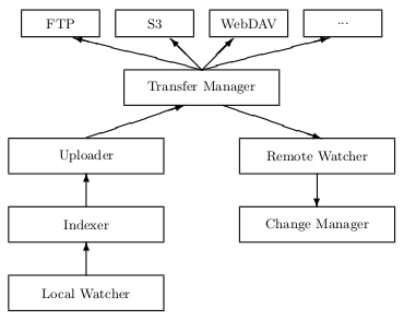 |
| Figure 4.1: Simplified Syncany architecture. When the local watcher detects changes in the watched folders, it passes the events to the indexer which then breaks the files into chunks. New chunks are uploaded by the uploader using a transfer manager. The remote watcher detects and downloads changes from the remote storage and passes them to the change manager which then applies these changes locally. |
The general architecture is straightforward: On the one hand, Syncany must watch the local file system for changes and upload altered files to the remote storage. On the other hand, it must handle changes made by other clients or workstations and apply them on the local machine. The Syncany architecture can be logically split according to these two process flows. The two processes are indicated on the left and right side of figure 4.1:
Local changes: For each user-defined Syncany folder on the local file system, the application registers a watch in the LocalWatcher. This watcher receives file system events from the operating system (OS): If a user creates, updates, moves or deletes a file in one of the watched folders, an event is triggered by the OS. This event is pre-processed by the watcher and then handed over to the Indexer. The indexer analyzes each file, splits it into chunks and adds metadata to the local database. If parts of the file have changed, it passes the according chunks to the Uploader which uses a TransferManager to upload them to the remote storage.
Remote changes: If other clients change a file on the remote storage, the local client must learn about these changes and apply them locally. Due to the heterogeneity of the repositories, the remote storage cannot actively notify clients that files have been updated. Instead, clients use the RemoteWatcher to poll for changes regularly. If new file entries or updates to existing entries have been found, the ChangeManager combines the clients’ file histories to one single history and identifies conflicts. It then applies these changes to the local file system.
The following sections give an overview over the most important concepts within Syncany.
4.5.1. Encryption
One of the core requirements of Syncany is the ability to use virtually any online storage without having to trust the owner of that storage. That is Syncany must ensure that data confidentiality is protected by any means. While this requirement can be easily achieved using modern encryption methods, the solution must consider other requirements and design goals.
There are a variety of ways to ensure that the desired security properties are protected. They use different cryptographic primitives to transform the plaintext files into cipher text before uploading them to the remote storage. Depending on the used method, it is possible to implement cryptographic access control [26,13], i.e. to cryptographically ensure that certain files can be read or written only with the respective access rights:
Single symmetric key: The easiest method is to use a single symmetric key, derived from a user password, to encrypt chunks and metadata. Users with the password can decrypt all the data in the repository with only one key. While this is a very convenient possibility to achieve confidentiality, it is vulnerable to cryptanalysis if enough chunks are analyzed.
Salted symmetric key: Similar to the single symmetric key method, this method uses one password to encrypt chunks and metadata, but salts the key with the checksum of each individual chunk (or any other value known to the client). This makes attacks on the key more difficult because it effectively encrypts each chunk with a different key. Users still have to remember only one password, but the system can create a key for each chunk. All users owning the password would hence be able to read/write all files.
Random symmetric keys: Instead of creating a key from a single password, this method creates a random key for each chunk and stores the value in the metadata. The client must look up the key in the metadata to encrypt/decrypt the respective chunks. Due to the additional random key, this method requires significant per-chunk storage overhead.
Asymmetric keys: The symmetric key methods grant all users with a valid key full access to all files and folders. Asymmetric cryptography, however, uses different keys to encrypt/decrypt data and can be used to implement multi-user support using cryptographic access control. Each client has its own key pair and encrypts files with a random symmetric key. This symmetric key is then encrypted with the public key of all clients with full access. If a client wants to decrypt a file, it has to first decrypt the symmetric chunk key with its own private key and can then decrypt the chunk.
The current architecture of Syncany uses a salted symmetric key based on the user password. There is no multi-user support and clients with the password have full read/write access to the repository. While this concept does not allow limiting access to a subset of users, it minimizes the computation required by the client and reduces complexity. The concept of a password is much easier to understand for end users and thereby matches the ease-of-use principle more than the asymmetric variant.
4.5.2. Versioning Concept
One of the requirements of Syncany is to allow versioning of files – in particular to allow restoring older file versions from the remote storage. Since the files and folders in the repository need to be encrypted and multiple storage types must be supported, none of the currently available version control systems are suitable. Syncany can hence not use any existing versioning mechanisms, but has to provide its own versioning system.
In contrast to traditional versioning software, Syncany must not support the full breadth of features and commands, but instead only focuses on what is required for its specific use case. In particular, Syncany’s versioning mechanism does not need to support the concepts of tags, branches or file merging. Instead, it rather focuses on tracking the version of a file as well as detecting and resolving conflicts.
Deduplication vs. Delta Compression: As indicated in chapter 2.2, most revision control software use snapshots and delta compression [58] to record changes between file revisions. This works very well for text files and satisfactory for binary files, but has significant disadvantages. When a file is changed locally and committed to a repository, the VCS must calculate the difference between the two revisions. To do that, it needs both versions of the file on the same machine. That is the VCS must (1) either upload the local file to the remote repository and then compare it with the old version or (2) keep a second copy of the old file on the local file system.
In the first case, it must transfer the entire new file even if only a single byte has changed. This potentially consumes enormous amounts of bandwidth and thereby defeats the purpose of the delta compression concept. An example that uses this variant is CVS.
In the latter case, the VCS effectively has to store each file twice on the local machine: the working copy as well as the complete history of the file. In the worst case, this requires up to double the amount of disk space. Examples that behave like this are Subversion and Bazaar.1 Both variants are acceptable if the upload bandwidth is sufficient and local disk space is not an issue. If, however, large files are to be stored in the repository, deduplication is more suitable than delta compression based VCS. Instead of having to compare the old version of the file with the new version, it creates chunks by using the locally available file and only uploads new chunks to the remote repository. That is it does not need an old version to compare, but only requires the newest file as well as a list of existing chunks. This method avoids having to upload the whole file and eliminates the need to store the entire change history locally.
Taking the requirement of client-side encryption into consideration, this disadvantage of delta compression becomes even more evident. In an encrypted VCS, the binary diffs stored in its repository have to be encrypted as well. That is if a file gets updated locally, the diff operation not only requires the version history to be read, but also implies several decryption operations prior to it. Since this has to be done for all altered files and every commit operation, the impact on performance would be significant.
As a consequence of the issues listed above, Syncany’s versioning system uses deduplication rather than delta compression: It breaks new or updated files into chunks and stores their identifiers in its local database. Each file consists of a set of chunks in a specific order. When small parts of a file change, the majority of the chunks are still identical. Syncany only has to upload the chunks that overlap with the updated parts of the file. The details of the deduplication algorithms are discussed in chapter 5.
Optimistic vs. Pessimistic Versioning: As soon as more than one person works with the same repository, there is a good chance that they accidentally update the same file in their local working copies. Once the clients commit their changes, the system has to deal with different versions of the same file. There are two commonly known solutions to handle this situation. The system either (1) locks the remote file while it is being written and thereby avoids conflicts in the repository or (2) it allows all clients to write the new file and resolves the issues at some later stage.
The first case is known as lock-modify-unlock in revision control or pessimistic replication in distributed systems [1,53,55]. In this model, the system locks the remote file while one client writes its changes and releases the lock once the write operation is complete. That is the repository ensures that only one client can make changes to a file at a time. This model pessimistically assumes that concurrent updates and conflicts happen regularly. While it avoids multiple versions of the same file in the repository, it relies on synchronous calls and blocks other clients during updates.
The latter case is known as copy-modify-merge in revision control or optimistic replication in distributed systems [1,77,53]. Instead of locking the repository, this model assumes that conflicts will occur only rarely and hence explicitly allows concurrent write access to the repository by different clients. The repository temporarily stores all file versions and later resolves problems by merging the changes into the working copies of the clients. This model has significant advantages over the pessimistic approach. Optimistic algorithms offer a greater availability of the system because they never have to lock files of file sets. Users work independent from each other since they do not have to rely on other users to release the lock. Instead, they commit their changes and get a quick response from the system. In addition to the improved usability and response time, optimistic systems have a higher scalability than pessimistic systems, because operations are asynchronous. This allows a large number of users/replicas to access the same system concurrently [53,77].
Syncany is based on the copy-modify-merge paradigm: In addition to the above mentioned advantages, an optimistic approach matches the purpose of the software better than a pessimistic one. Due to its asynchronous nature, it allows a more responsive user experience and can deal with variable client connectivity. Unlike most versioning software, Syncany never assumes that the local copy of files is in a final committed state. Each client keeps its own history and frequently compares it to the other clients’ histories. This approach is particularly useful because there is no central instance for coordination or locking. Details on this concept are explained in the next section.
4.5.3. Synchronization
The synchronization algorithm is one of Syncany’s core elements. Its responsibility is to detect file changes among participating workstations and to bring them to the same state. This particularly includes what is known by most file synchronizers as update detection and reconciliation [57,51,52,53,54].
Update detection is the process of discovering where updates have been made to the separate replicas since the last point of synchronization [57]. In state-based synchronizers [50] such as Unison or rsync, this is done by comparing the file lists of all replicas. The result is a global file list created by merging the individual lists into one. In trace-based synchronizers, update detection is based on the trace log of the replicas. Instead of a global file list, they generate a global file history based on the individual client histories. It typically compares histories and detects new file versions. Update detection must additionally detect conflicting updates and determine the winner of a conflict.
Once the global file list/history has been created, it must be applied to the local workstation. This is done in the reconciliation phase, which usually downloads new files, deletes old files and moves renamed files.
Due to Syncany’s versioning requirements, it detects updates via trace logs (file histories) of the individual clients. Histories of the participating clients are analyzed and compared to each other based on file identifiers, file versions, checksums and local timestamps. Syncany follows the optimistic replication approach. Clients populate their updates to the repository under the assumption that conflicts do not happen regularly. If a conflict occurs, each individual client detects it based on the trace log and determines a winner. The winning version of a file is restored from the repository and the local conflicting version is populated to the repository under a different name.
4.5.4. Storage Abstraction and Plugins
Unlike related software such as distributed file systems or versioning software, Syncany does not rely on a single type of storage, but rather defines a minimal storage interface, which makes it possible to support very heterogeneous storage types. Each supported storage is encapsulated in a plugin and must implement the generic methods upload, download, list and delete. This is a well-known approach for storage abstraction [6,16].
Each of these plugins can be used by Syncany in a very homogeneous way and without having to individually handle the different behavior of the storage types. The storage API mainly defines the exact behavior of these methods and thereby ensures that the plugins behave identically, even if they operate on entirely different protocols. Among others, the API defines the following behavior:
All operations must be synchronous.
All operations must automatically connect or reconnect (if necessary).
All operations must either return a valid result or throw an exception.
File entries returned by the list -operation must belong to the repository and match a certain file format.
The repository must always be in a consistent state.
The main advantage of this approach is obvious: Due to the fact that plugins must only implement a very small set of generic operations, almost anything can be used as storage. This is not limited to typical storage protocols such as FTP or WebDAV, but can be extended to rather unusual protocols such as IMAP or even POP3/SMTP.
Even though this is a great advantage, the list of incompatibilities among the different protocols is long: Traditional storage protocols such as NFS or WebDAV, for instance, support multiple users and can define read/write support for different folders depending on the user. IMAP, however, has no possibility to limit access to certain folders. Similarly, CIFS supports other file permissions than NFS and FTP behaves differently on transfer failures than Amazon S3.
Even though the minimal storage interface solves these issues, it also strongly limits the potential functionalities of the remote storage server and thereby also of the application – especially in terms of supported file size, authentication and multi-user support. The storage plugins must be able to deal with these differences and behave identically independent of the underlying protocol.
» Next chapter: Implications of the Architecture
- 1 These results have been acquired by monitoring local and remote disk usage as well as bandwidth in the following command sequence: (1) Commit a large binary file to the VCS, (2) append a single byte to the file, (3) commit again.
Download as PDF: This article is a web version of my Master’s thesis. Feel free to download the original PDF version.
5. Implications of the Architecture
After discussing related research and giving an overview of the Syncany architecture, this chapter focuses on optimizing the bandwidth and storage utilization. It discusses the implications of the software architecture on the storage mechanisms and explores their trade-offs.
In particular, it examines how the concepts used within Syncany (e.g. deduplication and storage abstraction) affect the bandwidth consumption of the application and how it impacts the local computing resources.
The chapter then discusses the various existing possibilities of the algorithm design and introduces the relevant parameters. Before finally discussing different algorithm configurations and their characteristics, it briefly explains the concept of multichunks.
5.1. Implications of the Syncany Architecture
The Syncany architecture as discussed in chapter 4 has direct implications on the possible variations of the deduplication mechanisms. Among others, it affects encryption and bandwidth consumption. The following sub-sections elaborate on the strongest of these effects.
5.1.1. Encryption, Deduplication and Compression
One of Syncany’s assumptions is that the remote storage cannot be trusted. Since public cloud resources could be used as storage, this is a valid assumption. As briefly discussed in chapter 4.5.1, Syncany uses symmetric key encryption as a countermeasure. By encrypting data before uploading it, data confidentiality can be maintained.
If encryption was the only data-altering step, the data transformation process would only have to transform plaintext into ciphertext. However, since deduplication and compression mechanisms are also involved, the process is more complicated. Encryption transforms data into a pseudo-random ciphertext that changes significantly even if only a few bytes of the source data change. Even for very similar files, the corresponding encrypted documents are most likely very different. In fact, if two source files are identical, their ciphertext is different (unless the salt is identical). Considering that deduplication exploits long sequences of identical bytes, it is obvious that it does not perform well on encrypted data. Consequently, combining the two technologies is not trivial [41]. There are at least two solutions to this issue:
The first possibility is to use convergent encryption, a cryptosystem that produces identical ciphertext files from identical plaintext files [33]. Unlike other encryption mechanisms, this variant allows the use of deduplication on the ciphertext, because for a given sequence of bytes, the output is always the same. However, since the generated cipher text is the same given a specific input, it makes cryptanalysis easier and thereby reduces the overall security of the system.
The second option is to perform deduplication before the encryption [41], i.e. to break files into chunks and afterwards encrypt them individually. Since the chunk checksums are generated before the encryption, the deduplication process is not interfered with, but the resulting data is still encrypted. However, even though this is a viable option, the non-obvious problem is the overhead created by the encryption of each chunk. Encrypting a larger number of chunks needs more time than encrypting one chunk of the same size. Similarly, it creates a higher byte overhead in the ciphertext. Encrypting 1 GB with AES-128 in 1 MB blocks, for instance, only creates an overhead of 16 KB in total (16 bytes per chunk). Using 8 KB chunks for the same data, the byte overhead is 2 MB.1
Even though the overhead is not significant on its own, it must be considered in combination with other metadata such as chunk checksums or versioning information. Additionally, depending on the storage type, chunks might not be stored in raw binary format, but using inflating encoding mechanisms such as Base64.
Having that in mind, the best option to optimize disk usage is to combine the unencrypted chunks into larger chunks and then encrypt them together as if they were a single file. This reduces the data overhead and minimizes the required time. This concept is further described in section 5.1.3.
5.1.2. Bandwidth Consumption and Latency
Syncany stores chunks and metadata on the remote storage using a minimal storage interface (as described in section 4.5.4). This lightweight API allows using almost anything as storage, but at the same time creates problems with regard to deduplication, concurrency control and change notification – and thereby strongly impacts the bandwidth consumption of the application.
Unlike most file synchronizers and versioning systems, Syncany’s architecture does not include any intelligent servers, but instead only relies on a simple storage system. Unison and rsync, for instance, perform processing tasks on both participating systems. They generate file lists and checksums on both machines and exchange the results. Not only does this limit the processing time required by each of the machines, it also conserves bandwidth.
Syncany cannot rely on information created by the remote system, but instead has to download the complete file histories of all participating clients. Depending on the number of users, this can have a significant impact on the amount of data that needs to be downloaded (and processed) by each client.
With regard to change notification, the server cannot actively notify its clients of any changes on the files. Syncany must instead use alternative methods to determine if updates are available. Given the heterogeneity of the storage types, the easiest way to do this is polling, i.e. to frequently query the remote storage for changes. In comparison to push-based notifications, polling negatively affects the liveness of the updates, but more importantly potentially consumes significant bandwidth. Assuming a polling interval of ten seconds and an efficient organization of the repository on the remote storage,2 polling consumes a few dozen kilobytes per minute. If the repository is not efficiently organized, the polling bandwidth can rise up to a few hundred kilobytes per minute. Depending on the amount of users and whether traffic is costly, polling can have significant impact on the overall bandwidth and cost.
Another factor that strongly influences the required overall bandwidth consumption is the individual protocol overhead. Due to the fact that Syncany works with different storage protocols, it cannot rely on an efficient data stream, but has to consider the heterogeneous behavior of these protocols. Among others, they differ in terms of connection paradigm, encryption overhead and per-request overhead:
- Connection paradigm: Communication protocols can be divided by whether or not they need to establish a connection to the remote machine before they can communicate. While connection-oriented protocols need to do so, connectionless protocols do not. Connection-oriented protocols (such as SSH or FTP) typically have a higher one-time overhead, because a session between the two machines must be established before the actual payload can be sent. While this usually means that subsequent requests are more lightweight and have a smaller latency, it also implies a consequent connection management on both sides. Requests in connectionless protocols (such as HTTP/WebDAV or other REST-based protocols) are usually more verbose because they must often carry artificial session information. This not only negatively impacts the bandwidth, but also often the latency of connections.
Even though the Syncany storage API works with both paradigms, it requires the plugins to handle connections on their own. That is especially connection-oriented protocols must disguise the connection management and behave as if they were connectionless.
Encryption overhead: If the communication protocol is encrypted using TLS, the initial connect-operation is preceded by the transport-level TLS handshake and the actual payload is encrypted with a session key. While TLS ensures that all communication between the two machines is secure, it also adds reasonable overhead to the connection: The handshake exchanges certificates, cipher suites and keys and thereby increases the latency before the first payload can be sent. Because subsequent messages are encrypted with a symmetric key, their overhead and latency is not significant.
Per-request overhead: The per-byte overhead of request and response headers differs greatly among the different application protocols. While distributed file system protocols such as NFS or CIFS have very lightweight headers and messages, many others are rather verbose. Especially SOAP or REST-based protocols have very descriptive headers and often require inflating encodings for binary data. If an IMAP mailbox is used as storage, for instance, payload is typically Base64 encoded and hence grows by about 30%. Another example is the overall size of a list -request and response in the FTP and WebDAV protocol: While retrieving a file list via FTP only requires an overhead of 7 bytes, WebDAV needs at least 370 bytes per request/response cycle.3
These protocol-dependent properties imply that Syncany must adapt to counteract the heterogeneity in bandwidth consumption and latency. In particular, it must try to reduce the total amount of requests in order to minimize the overall byte overhead and latency. A key factor to regulate the request count is the average chunk size: Assuming that each chunk is stored in a separate file, increasing the average chunk size reduces the per-chunk bandwidth overhead. Conversely, the more chunks must be transferred, the higher the overall overhead.
Assuming that upload -requests have a similar overhead as list requests, uploading 1 GB of data (with an average chunk size of 8 KB) would only require a total overhead of (1 GB / 8 KB) × 7 bytes = 875 KB for FTP, whereas for WebDAV, the overhead would be about 46 MB. With an upload bandwidth of 70 KB/s that would be 11 minutes for WebDAV, compared to only 12 seconds for FTP.4
5.1.3. Reducing Requests by Multichunking
Other synchronization software reduces the request count by combining many small files into a single file stream. rsync, for instance, uses only one data stream per transfer direction. Due to the fact that the software runs on both machines, it can split the stream into individual files on retrieval. Instead of having to send one request per file, it only sends two requests in total (constant time).
While this technique works if the storage host can perform intelligent tasks, it does not work with Syncany’s storage concept. Due to its abstract storage interface, uploaded data cannot be processed or transformed on the remote storage, but always stays unaltered. In particular, because files cannot be split, combining all of them into a single large file before upload is unreasonable.
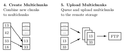 |
| Figure 5.1: The multichunk concept extends the deduplication process (cf. figure 3.1) by combining the resulting chunks in a larger container. It thereby minimizes the amount of upload and download requests. |
This thesis proposes a solution to this issue: By adding many chunks to a large container, a multichunk, it reduces the per-request overhead significantly. Instead of storing each chunk individually, many chunks are combined into a single multichunk and then uploaded to the remote storage. Due to the drastic reduction of files, the amount of requests can be reduced significantly and thereby speed up the upload (and download) of a certain file set. For the example above, combining 8 KB chunks into 512 KB multichunks reduces the WebDAV overhead to about 720 KB (10 seconds) and the FTP overhead to only 14 KB (200 ms).
However, while the multichunking concept reduces the amount of requests, it increases the amount of required metadata. Without multichunks, the index must only contain a list of chunks as well as a mapping between files and chunks. With multichunks, an additional mapping between multichunks and chunks is necessary to identify the file a chunk is stored in.
Another great disadvantage of the multichunking concept is that in order to retrieve a single chunk from the remote storage, Syncany must download the entire multichunk which contains this chunk. In a worst case scenario, even if only a single chunk is needed from a multichunk, the complete multichunk must be retrieved. In the example above, the retrieval of an 8 KB chunk would imply the download of a 512 KB chunk – producing a download overhead of 502 KB (98%).
5.2. Design Discussion
The apparent goal of the chunking algorithm is to reduce the amount of required storage space on the remote repository as well as to maximize the required upload and download bandwidth. While these goals are the primary objective, they cannot be examined in an isolated environment. Since the software will be running on an end user client, the proposed mechanisms must make sure that they do not disturb the normal execution of other applications – especially in terms of processing time and bandwidth usage. On the other hand, they must not slow down the indexing operation or negatively affect the system load.
The mechanisms developed in the scope of this thesis must not be optimized for a general purpose, but should rather be tailored to the scope and architecture of Syncany. That means that they have to consider Syncany’s unique properties such as encryption or storage abstraction.
Additionally, it is important to mention that even though the goal is to minimize disk utilization on the remote storage, this goal is not meant to be reached by the first upload, but rather within a well-defined period of time. That is the storage optimizations to be discussed do not aim on reducing the size of a single file set, but rather try to exploit the similarities between two or more versions of the same set of files. Even though they can in some cases already reduce the total file size with the first index process, the best results are to be expected for file sets with regular, but comparably small changes. Examples include the folders with office documents or e-mail archive files.
The following sections elaborate the possible variations of the algorithms and their relevant parameters. Since the efficiency of the deduplication process strongly depends on how these parameters are combined, a primary goal of the experiments below is to find the optimal configuration of these parameters with regard of the data typically found in Syncany folders.
5.2.1. Chunking Parameters
Arguably one of the most important aspects is the chunking mechanism, i.e. the method by which files are being broken into pieces to identify duplicate parts among different files. Not only can this algorithm influence the deduplication ratio, it can also have a significant impact on the indexing speed, local disk utilization and other factors.
| Chunking | Fingerprinting | Chunk Size | Chunk ID | Indexing |
| Whole File (SIS) | None (fixed only) | 2 KB | MD5 | In-Memory (Flat) |
| Fixed Offset | Adler-32 | 4 KB | SHA-1 | In-Memory (Tree) |
| Variable TTTD | PLAIN | 8 KB | ... | Persistent Database |
| Variable Kruus | Rabin | 16 KB | Extreme Binning | |
| Type-Aware | 32 KB | ... | ||
| ... |
Table 5.1: Possible configuration parameters for chunks. Only values in bold font are considered in the experiments in chapter 6.
Many of the possible chunking options have been discussed in chapter 3.4. The most important parameters of how to break files into chunks are chunking method, fingerprinting mechanism, chunk size, chunk identity hash function as well as index structure. A selection of the possible values is depicted in table 5.1.
The average chunk size is expected to have the biggest impact on the efficiency of the deduplication process. In general, small chunks lead to better space savings than big chunks, but need more processing time and generate more metadata. Common chunk sizes in commercial deduplication systems are 2 – 64 KB.
Another major factor is the chunking method: Since it defines the general chunking algorithm, it decides whether files are broken into chunks at well-defined offsets (fixed-size), based on the file content (variable-size), file type (type aware) or not at all (SIS). For the content-based chunking methods, both the chunking method and the fingerprinting mechanism are responsible for finding the file breakpoints.
The last two parameters (chunk identity function and indexing method) have no influence on the deduplication process, but rather on the size of the metadata, the indexing speed and the processing time. Consequently, they also affect the bandwidth consumption when uploading/downloading chunks to the remote storage: The chunk identity function generates a hash over the chunk contents. Because chunks are identified with this function, it must be resistant against collisions. At the same time, its bit-length affects the amount of generated metadata. The indexing mechanism (in-memory vs. on-disk) only affects the indexing speed. For the expected amount of data to be handled by Syncany, an in-memory index is the best option, because it avoids time consuming disk lookups.
5.2.2. Multichunking Parameters
The multichunking concept, i.e. the combination of many chunks into a large file container, minimizes the overall transfer overhead by reducing the total amount of files and thereby the overall amount of upload/download requests. While the general idea is straightforward, the concept allows for some variation in the container format as well as on how the container is post-processed before storing/uploading it. Table 5.2 shows a limited set of possible parameters.
| Container | Min. Size | Compression | Encryption | Write Pause |
| None | 125 KB | None | None | None |
| ZIP | 250 KB | Gzip | AES-128 | 30 ms |
| TAR | 500 KB | Bzip2 | AES-192 | 50 ms |
| Custom | 1 MB | LZMA/7z | AES-256 | ... |
| ... | ... | Deflate | 3DES-56 | |
| ... | 3DES-112 | |||
| ... |
Table 5.2: Possible multichunk configuration parameters. Only values in bold font are considered in the experiments in chapter 6.
A multichunk container can be any composite file format. It can either be an existing format such as TAR or ZIP or a custom format specifically designed for Syncany. While known file formats are more convenient in terms of development (because chunks can be simply added as file entries), they produce larger output files than a customized slimmed-down file format (particularly because they store additional metadata and chunk identifiers need to be encoded). The experiments only consider a well-defined Syncany specific format.
In order to influence the actual amount of requests, the most important parameter is the minimum size of the container file. Due to the fact that larger container files lead to fewer upload/download requests, it is generally more desirable to produce large multichunks. However, because multichunks cannot be extracted on the remote storage, downloading a single chunk always implies downloading the entire corresponding multichunk. Hence, the goal is to find a reasonable trade-off between multichunk size and the amount of unnecessarily downloaded bytes. The experiments analyze this trade-off by looking at the reconstruction overhead and bandwidth.
Apart from the minimum size parameter, the type of post-processing also influences the resulting multichunk. Before a multichunk is uploaded to the remote storage, Syncany must encrypt the data and might perform additional compression.
In order to encrypt a multichunk, any symmetric encryption mechanism can be used (cf. chapter 4.5.1). Besides the level of security they provide, the possible algorithms (such as AES or 3DES) mainly differ in terms of processing time and the amount of generated output data. While these factors affect the overall bandwidth consumption and the indexing speed, they are not relevant for optimization purposes, but rather a security trade-off the user must decide. The experiments in this thesis only use AES-128.
In contrast, the choice of the compression algorithm should not be a user decision, but can be chosen to make the resulting multichunk size minimal and the processing time acceptable. The trade-off in this case is not security, but the amount of processing resources used by the algorithm. If compression is used, writing a multichunk creates significant CPU time overhead (compared to no compression). The experiments are limited to the options no compression, Gzip and Bzip2. 5
Due to the many CPU intensive processing steps of the chunking algorithm (chunking/fingerprinting, indexing, encryption, compression), the CPU usage is potentially very high and most certainly noticeable to the user. Because it is not possible to skip any of these steps, artificial pauses are the only option to lower the average CPU load. Instead of writing one multichunk after the other, the algorithm sleeps for a short time after closing the multichunk. Even though this technique helps limiting the CPU utilization, it also slows down the indexing speed. The experiments test sleep times of 0 ms (no pause) and 30 ms.
5.3. Algorithm Discussion
Given the set of configuration parameters discussed above, the chunking and indexing algorithm has a very similar structure for all the different values. In fact, it can be generalized and parameters can be passed as arguments. The result is a very simple chunking algorithm, which (a) breaks files into chunks, (b) identifies duplicates and (c) adds new chunks to the upload queue.
Listing 5.1 shows a simplified version of this generic algorithm (disregarding any encryption, compression or multichunking mechanisms):
void index(files, config):
  for each file in files do:
    chunks = config.chunker.create_chunks(file)
    while chunks.has_next() do:
      chunk = chunks.next()
      if index.exists(chunk.checksum): // existing chunk
        existing_chunk = index.get(chunk.checksum)
        ...
      else: // new chunk
        index.add(chunk)
        upload_queue.add(chunk)
        ...
Listing 5.1: Generic chunking algorithm (pseudo code).
The algorithm’s input parameters are the files to be indexed as well as the chunking parameters (config). Any of the chunking parameters (such as chunking method or chunk size) are comprised within the config.chunker object. The algorithm breaks each file into individual chunks (line 3) and checks if each of them already exists in the index. If it does (line 6), the existing chunk can be used. If it does not (line 9), the chunk is added to the index and queued for uploading.
Depending on the desired chunking options, a corresponding chunker has to be created. If, for instance, fixed-size chunking with a maximum chunk size of 8 KB and MD5 as identity function shall be used, chunking and indexing a given set of files can be done as shown in listing 5.2. In order to use other chunking mechanisms and parameters, the configuration needs to be adjusted with the according parameters.
config = { chunker: new fixed_size_chunker(8000, "MD5") }
index(files, config)
Listing 5.2: Example algorithm call using fixed-size 8 KB chunks with a MD5 chunk identity function.
While this algorithm describes the basic deduplication mechanisms, it does not encompass the concepts of multichunks, encryption or compression (cf. table 5.2). To allow the use of these concepts, it must be extended accordingly:
- Multichunks: To allow multiple chunks to be stored inside a single container (or multichunk), the algorithm must keep track of the currently opened multichunk and close it if the desired minimum multichunk size is reached.
- Transformation: Before writing the multichunk to the local disk (or uploading it), encryption and compression must be performed. Because both of them alter the original data stream, they can be classified as transformation.
- Write pause: After closing a multichunk, a short sleep time might be desired to artificially slow down the chunking process (and thereby limit the CPU usage).
The new multichunking algorithm in listing 5.3 encompasses all of these changes:
void index_multi(files, config):
  for each file in files do:
    chunks = config.chunker.create_chunks(file)
    while chunks.has_next() do:
      chunk = chunks.next()
      if index.exists(chunk.checksum):
        existing_chunk = index.get(chunk.checksum)
        ...
      else:
        if multichunk != null and multichunk.is_full(): // close multi
          multichunk.close()
          upload_queue.add(multichunk)
          multichunk = null

        if multichunk == null: // open multi
          multichunk = config.multichunker.create(config.transformerchain)

        index.add(chunk, multichunk)
        multichunk.write(chunk)
        ...

    if multichunk != null: // close last multi
      multichunk.close()
      upload_queue.add(multichunk)
Listing 5.3: Generic multichunking algorithm (pseudo code).
While this algorithm behaves identically in case the chunk already exists in the index, it has a different behavior for new chunks (highlighted in dark gray, lines 10-24): Instead of queuing each individual chunk for upload, this algorithm adds it to the currently opened multichunk (line 19). If the multichunk is full, i.e. the minimum multichunk size is reached, it is queued for upload (lines 10-13).
After closing a multichunk, the algorithm creates a new one using the configuration parameters defined by the config argument (lines 15-16). This particularly comprises instantiations of a multichunker (such as a TAR or ZIP based multichunker), as well as a transformerchain (e.g. a combination of Gzip and a AES cipher).
Continuing the example from listing 5.2, the following configuration additionally uses 512 KB TAR multichunks, a 15 ms write pause, Gzip compression and AES encryption (figure 5.4):
config = {
  chunker: new fixed_size_chunker(8000, "MD5"),
  multichunker: new tar_multichunker(512*1000, 15),
  transformerchain: new gzip_compressor(new cipher_encrypter(...))
}

index_multi(files, config)
Listing 5.4: Example algorithm call using fixed-size 8 KB chunks, a MD5 chunk identity function, 512 KB TAR multichunks, a 15 ms write pause and Gzip compression.
This generic algorithm allows for a very simple comparison of many different chunking and multichunking configurations. The experiments in this thesis use the algorithm and a well-defined set of configuration parameters to test their efficiency and to identify the best configuration for Syncany.
- 1 This has been tested and verified by the author.
- 2 The current version of Syncany does not always efficiently organize files on the remote storage. Instead, it stores chunks and metadata without any hierarchy in a flat list of files.
- 3 Tested by the author. The calculation does neither include the overhead generated by the underlying protocols (TCP/IP), nor the per-entry bytes. It only includes the fixed amount of header and payload bytes. For FTP, this is simply the command
LIST -a. For WebDAV, this includes thePROPFINDrequest and a 207 Multi-Status response. - 4 Since Syncany is an end-user application, upload bandwidth in this example is assumed to be typical DSL upload speed.
- 5 Due to the high number of other parameters and the resulting number of possible configurations, only very few options can be compared within this thesis.
Download as PDF: This article is a web version of my Master’s thesis. Feel free to download the original PDF version.
6. Experiments
The experiments in this thesis analyze and compare the different possible configurations based on the described algorithm and based on a set of carefully chosen datasets. The overall goal of all experiments is to find a good combination of configuration parameters for the use in Syncany – good being defined as a reasonable trade-off among the following goals: * The temporal deduplication ratio is maximal * The CPU usage is minimal * The overall chunking duration is minimal * The upload time and upload bandwidth consumption is minimal * The download time and download bandwidth consumption is minimal The scope of the experiments focuses on the three main phases of Syncany’s core. These phases strongly correlate to the architecture discussed in chapter 4.5. They consist of the chunking and indexing phase, the upload phase as well as the download and reconstruction phase (figure 6.1).
 |
| Figure 6.1: The experiments aim to optimize Syncany's core phases in terms of deduplication ratio, processing time and bandwidth consumption. The main focus is on the chunking and indexing phase. |
Due to the high significance of the chunking and multichunking mechanisms, the biggest part of the experiment focuses on finding the optimal parameter configuration and on analyzing the interrelation between the parameters.
The following sections describe the surrounding conditions of the experiments as well as the underlying datasets.
6.1. Test Environment
Since Syncany runs on a client machine, all experiments were performed on normal user workstations.
The test machine for experiment 1 and 3 is a desktop computer with two 2.13 GHz Intel Core 2 Duo 6400 processors and 3 GB DIMM RAM (2x 1 GB, 2x 512 MB). It is located in the A5 building of the University of Mannheim, Germany. The machine is connected to the university network.
Since the setting for experiment 2 requires a standard home network connection, it is performed on a different machine. The test machine for this experiment is a Lenovo T400 notebook with two 2.66 GHz Intel Core 2 Duo T9550 processors and 4 GB DDR3 SDRAM. During the tests, the machine was located in Mannheim, Germany. The Internet connection is a 16 Mbit/s DSL, with a maximum upload speed of about 75 KB/s and a maximum download speed of 1.5 MB/s.
6.2. Parameter Configurations
The numerous possibilities to combine the parameters (as discussed in section 5.2) makes a complete analysis of all the combinations on all datasets unfeasable. As a consequence, the configurations chosen for this experiment are rather limited.
With the selection as indicated by the bold values in tables 5.1 and 5.2, there are in total 10 possible parameters. In particular, there are 12 chunkers, 4 multichunkers and 3 transformer chains, totalling to 144 different configurations. The following list is an excerpt of the configurations analyzed in this thesis. Appendix A shows the complete list:
* Custom-125-0/Fixed-4/Cipher

* Custom-125-0/TTTD-4-Adler32/Cipher

* Custom-125-0/TTTD-4-PLAIN/Cipher

* Custom-125-0/TTTD-4-Rabin/Cipher

*...
The syntax of the configuration string is as follows: Multichunker/Chunker/TransformationChain. Hyphens indicate the parameters of each of the components.
The syntax of the multichunker is represented by the type (always Custom), the minimum multichunk size (here: 125 KB or 250 KB), as well as the write pause (0 ms or 30 ms).
The chunker’s parameters include the type (Fixed or TTTD), the chunk size (4 KB – 16 KB) as well as the fingerprinting algorithm (only TTTD: Adler-32, PLAIN or Rabin).
The transformation chain’s parameters consist of a list of transformers (encryption and compression) in the order of their application. Possible values are Cipher (encryption), Gzip or Bzip2 (both compression).
6.3. Datasets
The datasets on which the experiments are conducted have been carefully chosen by the author based on the expected file types, file sizes, the amount of files to be stored as well as the expected change patterns to the files. To support the selection process, additional information has been collected from a small number of Syncany users and developers (35 participants). Appendix B shows details about what users were asked to do and what was analyzed. In particular, the pre-study collected the following data:
* Distribution of certain file types by size/count (e.g. JPG or AVI)

* Number/size of files that would be stored in a Syncany folder
Even though the results of this study are not representative of typical Syncany user data,1 they help by getting a better understanding of what data Syncany must expect. In particular, the data can be used to optimize the algorithms and/or the configuration parameters.
6.3.1. Pre-Study Results
This section briefly summarizes the results of the pre-study.
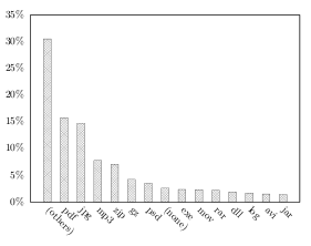 | 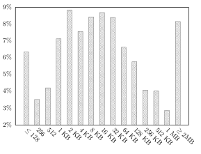 |
| Figure 6.2: Distribution of file types in the users' Syncany folder by size | Figure 6.3: Distribution of file sizes in the users' Syncany folder by size |
File sizes: The size distribution of the files in the users’ Syncany folders shows that over half of the files’ sizes range from 512 bytes to 32 KB. About 75% are smaller than 128 KB and only very few (8%) are greater than 2 MB (cf. figure 6.3).
Total size distribution: The total size of the users’ Syncany folders ranges from a few megabytes (minimum 9 MB) to over 600 GB for a single user. Most of the users store no more than 3.5 GB (67%), but also about 19% store more than 6 GB. The median share size is 1.5 GB.
Number of files: The amount of files varies greatly between the users. Some users only store a few dozen files, others have over 200,000 documents in their Syncany folders. About 51% store less than 3.400 files and about 75% less than 27,500 files. Only 10% store more than 100,000 files in the Syncany folders. The median number of files is 3,085.
File types:2 There is a large variety of distinct file extensions in the users’ Syncany folders, many of which only occur very few times. Counting only those which occurred more than once (10 times), there are 2177 (909) distinct file extensions. If counted by file size, both PDF documents and JPG images each account for 15% of the users’ files. Another 30% consists of other file types (figure 6.2). When counting by the number of files, PDF files (JPG files) account for 10% (9%) of the users’ Syncany folders and office documents3 for about 8%.
6.3.2. Dataset Descriptions
Since the pre-study only captured a (non-representative) snapshot of the users’ potential Syncany folders, the datasets used for the experiments are only partially derived from its results. Instead, the actual datasets represent potential usage patterns and try to test many possible scenarios. In particular, they try to simulate the typical behavior of different user groups.
At time t0, each of the datasets consists of a certain set of files, the first version of the dataset. This version is then changed according to a change pattern – for instance by updating a certain file, adding new files or removing old files. Depending on the pattern, the dataset at time t can either differ by only very small changes or by rather big changes. Figure 6.4 illustrates a changing dataset over time. Each dataset version consists of a certain set of files. By altering one version of a dataset, a new version with new files is created.
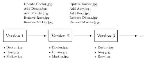 |
| Figure 6.4: Example of a dataset, updated by a user over time |
Consider a user working on an office document: If the document resides inside the monitored Syncany folder, it is very likely that changes to this document are rather small. If, however, the user only backs up the file in regular time intervals, changes are most likely bigger. Depending on the change pattern and file formats within a dataset, the deduplication algorithms are more or less effective. The following list briefly describes each of the datasets used for the experiments:
* **Dataset A** consists of a very small set of office documents which are gradually altered over time. Each dataset version at time t differs only by a single modification in one document. This dataset represents the usage pattern described above: A user works on a file and saves it regularly. Whenever the file is saved, the deduplication process is triggered by Syncany.

* **Dataset B** mostly contains file formats that are typically not modified by the user (such as JPG, PDF and MP3), but rather stay the same over time. With rare exceptions, subsequent dataset versions only differ by newly added files or by deleted files. This dataset represents a user group who mainly use Syncany to share files with others (or for backup).

* **Dataset C** contains a set of files that is composed of the 10 most frequent file types as found in the pre-study (by size). Each of the dataset versions differs by about 1--10 files from its predecessor. This dataset represents a daily-backup approach of a certain folder.

* **Dataset D** contains the Linux kernel sources in different versions -- namely all released versions between 2.6.38.6 and 3.1.2. Each of the dataset versions represents one committed version within the version control system. This dataset is used to test how the algorithms perform on regularly changed plain text data. Using the source code of large open source projects is a common technique to test the efficiency of deduplication algorithms on plain text data [[49](/blog/minimizing-remote-storage-usage-and-synchronization-time-using-deduplication-and-multichunking-syncany-as-an-example/#Reference49),[67](/blog/minimizing-remote-storage-usage-and-synchronization-time-using-deduplication-and-multichunking-syncany-as-an-example/#Reference67)].
| Dataset | Versions | Size | Files | Description | |
| A | Office documents | 50 | 5--9 MB | 24--25 | Collection of Microsoft Office and OpenOffice documents |
| B | Rarely modified | 50 | 400--900 MB | 700--1,900 | Collection of files that are rarely modified |
| C | Top 10 types | 50 | 100--150 MB | 230--290 | Collection of files based on the top 10 data types (by size) of the results of the pre-study |
| D | Linux kernels | 20 | 470--490 MB | 38,000--39,400 | Subsequent revisions of the Linux kernel source code |
Table 6.1: Underlying datasets used for the experiments.
Each of the experiments corresponds to one of Syncany’s core processes (as depicted in figure 6.1). The following sections describe each experiment and discuss their outcome.
6.4. Experiment 1: Chunking Efficiency
In order to reduce the overall amount of data, the efficiency of the chunking algorithm is the most important factor. The aim of this experiment is to find a parameter configuration that creates multichunks of minimal size, but at the same time does not stress the CPU too much.
The experiment compares the parameter configurations against each other by running the algorithms on the test datasets. It particularly compares runtime, processor usage, as well as the size of the resulting multichunks and index. This experiment helps analyzing the impact of each configuration parameter on the overall result of the algorithm. The goal is to find a configuration that matches the above aims (namely minimize result size, CPU usage and processing time).
The algorithm used for the experiment is very similar to the one described in chapter 5.3. In addition to the chunking and multichunking functionality, however, it includes code to create the index as well as mechanisms to calculate and measure the required parameters.
6.4.1. Experiment Setup
This experiment runs the Java application ChunkingTests on each of the datasets: It first initializes all parameter configurations, the chunk index, cache folders on the disk as well as an output CSV file. It then identifies the dataset versions of the given dataset (in this case represented by sub-folders) and finally begins the chunking and indexing process for each version.
The first version represents the initial folder status at the time t0. Each of the subsequent versions represent the folder status at time tn. In the first run (for t0), the index is empty and all files and chunks discovered by the deduplication algorithm are added. For subsequent runs, most of the discovered chunks are already present in the index (and hence in the repository) and do not need to be added.
For each version, the application records the index status and measures relevant variables. Most importantly, it records the size of the resulting multichunks, the CPU usage and the overall processing time using the current parameter configuration. Among others, each run records the following variables (for a detailed explanation of each variable see appendix C):
| totalDurationSec totalChunkingDurationSec totalDatasetFileCount totalChunkCount totalDatasetSize totalNewChunkCount totalNewChunkSize totalNewFileCount totalNewFileSize totalDuplicateChunkCount | totalDuplicateChunkSize totalDuplicateFileCount totalDuplicateFileSize totalMultiChunkCount totalMultiChunkSize totalIndexSize totalCpuUsage tempDedupRatio tempSpaceReducationRatio tempDedupRatioInclIndex | tempSpaceRedRatioInclIndex recnstChunksNeedBytes recnstMultChnksNeedBytes recnstMultOverhDiffBytes recnst5NeedMultChnkBytes recnst5NeedChunksBytes recnst5OverheadBytes recnst10NeedMultChnkBytes recnst10NeedChunksBytes recnst10OverhBytes |
Figure 6.5: List of variables recorded by the ChunkingTests application for each dataset version.
Each dataset is analyzed 144 times (cf. section 6.2). For each parameter configuration, the application analyzes all the versions for the given dataset and records the results in a CSV file. For a dataset with 50 dataset versions, for instance, 7,200 records are stored.
6.4.2. Expectations
Both literature and the pre-testing suggest that a deduplication algorithm’s efficiency strongly depends on the amount of calculations performed on the underlying data as well as on how much data is processed in each step. The CPU usage and the overall processing time is expected to increase whenever a configuration parameter implies a more complex algorithm or each step processes a smaller amount of data. Each of the configuration parameters is expected to behave according to this assumption.
This is particularly relevant for the chunking algorithm, the fingerprinting algorithm and the compression mechanism. As indicated in chapter 3.4, coarse-grained chunking algorithms such as SIS with their rather simple calculations are most likely less CPU intensive than algorithms analyzing the underlying data in more detail. The two algorithms Fixed Offset (lower CPU usage) and Variable TTTD (higher CPU usage) used in these experiments are expected to behave accordingly. In terms of chunking efficiency, TTTD is expected to outperform the fixed offset algorithm due to its content-based approach.
The fingerprinting algorithms Adler-32, PLAIN and Rabin all perform significant calculations on the data. However, while PLAIN is mainly based on simple additions, it is expected to use fewer CPU than the other two. Since Rabin uses polynomials in its calculations, it will most likely use the most CPU out of the three. In terms of their efficiency, literature suggests that PLAIN is more effective than Rabin [38]. Since Adler-32 is not referenced in deduplication research, no statements can be made about its efficiency, speed or CPU usage. The three fingerprinting algorithms compete with the fixed offset algorithm which performs no calculations, but breaks files at fixed intervals. This method (in experiments called None) is expected to have the lowest average CPU usage, temporal deduplication ratio and total chunking duration (fastest).
In addition to the chunking and fingerprinting, Syncany’s algorithm compresses the resulting multichunks using Gzip or Bzip2. Naturally, using compression is much more CPU intensive than not using any compression at all (None). Hence, both processing time and CPU usage are expected to be very high compared to the compression-free method. However, the filesize of the resulting multichunks is most likely much smaller when using compression.
In terms of chunking efficiency, the chunk size parameter is expected to have the greatest impact. A small chunk size amplifies the deduplication effect and thereby decreases the resulting total multichunk size. On the contrary, it increases the number of necessary iterations and calculations which leads to a higher CPU usage.
In addition to the configuration parameters, the chunking efficiency is expected to greatly vary depending on the underlying dataset. Generally, the composition of file types within a dataset as well as the size of the dataset is expected to have a great influence on the overall deduplication ratio. Datasets with many compressed archive files, for instance, are expected to have a smaller deduplication ratio than datasets with files that change only partially when updated. Large datasets supposedly have a higher deduplication ratio than smaller ones, because the chances of duplicate chunks are higher with a growing amount of files.
Depending on how often files within a dataset are changed (change pattern), the temporal deduplication ratio is affected: Many changes on the same files most likely lead to a higher ratio (many identical chunks), whereas adding and deleting new files to the dataset is expected to have no or little influence on the ratio. Generally, the longer a dataset is used by a user, the higher the ratio is expected to be.
6.4.3. Results
The experiment compared 144 configurations on the four datasets described above (44 GB in total). Overall, the algorithms processed 6.2 TB of data and generated nearly 50 million chunks (totalling up to 407 GB of data). These chunks were combined to about 2.3 million multichunks (adding up to 330 GB of data). The total chunking duration of all algorithms and datasets sums up to 61 hours (without index lookups, etc.) and to a duration of over 10 days for the whole experiment.
The following sections present the results for both the best overall configuration as well as for each of the individual parameters. They look at how the parameters perform in terms of CPU usage, chunking duration as well as chunking efficiency.
6.4.3.1. Chunking Method
The chunking method generally decides how files are broken into pieces. A chunking algorithm can either emit fixed size chunks or variable size chunks.
The results of the experiment are very similar to what was expected before. Generally, the TTTD chunking algorithm provides better results in terms of chunking efficiency (temporal deduplication ratio) than the Fixed algorithm. However, it also uses more CPU and is significantly slower.
Over all test runs and datasets, the average temporal deduplication ratio of the TTTD algorithms is 12.1:1 (space reduction of 91.7%), whereas the mean for the fixed-size algorithms is 10.8:1 (space reduction of 90.7%). Looking at the total multichunk sizes, the average space savings using TTTD are about 4.6% when comparing them to the fixed-size algorithms, i.e. the multichunks generated by TTTD are generally smaller than the ones by the fixed-size algorithms.
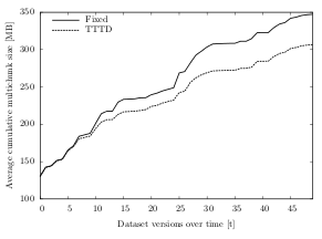 | 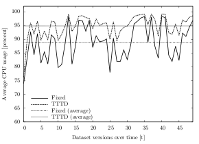 |
| Figure 6.6: Average cumulative multichunk size over time, compared by chunking algorithm (dataset A) | Figure 6.7: Average CPU usage over time, compared by the chunking algorithm (dataset C) |
For dataset C, the space savings of the variable-size algorithms are a lot higher than the average. The multichunks created with a TTTD algorithm are about 13.2% smaller than the ones using fixed-size algorithms. That equals to space saving of about 810 KB per run. Figure 6.6 illustrates this difference over time: Both TTTD and the fixed-size algorithms create about 130 MB of multichunks in the first run. However, the variable-size chunking algorithms save space with each dataset version in tn – totalling up to a difference of over 40 MB after 50 versions (306 MB for TTTD and 347 MB for the fixed-size algorithms).
In terms of CPU usage, the fixed-size algorithms use less processing time than the variable-size algorithms. On average, TTTD algorithms have a 3.6% higher CPU usage percentage (average of 93.7%) than the fixed-size ones (average of 90.0%). In fact, the TTTD CPU percentage is above the fixed-size percentage in almost every run. Figure 6.7 shows the average CPU usage while chunking dataset D using both fixed-size and variable-size algorithms. With a value of 94.8%, the TTTD average CPU usage is about 6% higher than the fixed-size average (88.8%).
Similar to the CPU usage, the less complex fixed-size chunking method performs better in terms of speed. However, while the CPU usage only slightly differs between the two chunking methods, the chunking duration diverges significantly. On average, the fixed-size algorithms are more than 2.5 times faster than variable-size algorithms. Over all datasets and runs, the average chunking duration per run for the fixed-size algorithms is about 4.1 seconds, whereas the average duration for the TTTD algorithms is 10.7 seconds. Depending on the underlying dataset, this effect can be even stronger: For dataset B, the fixed-size algorithms are on average 14.3 seconds faster than the TTTD algorithms, which is almost three times as fast (average per-run chunking duration of 7.8 seconds for fixed-size and 22.2 seconds for TTTD). After 50 runs, this time overhead adds up to almost 12 minutes (6.5 minutes for fixed-size, 18.5 minutes for TTTD).
6.4.3.2. Fingerprinting Algorithm
The fingerprinting algorithm is responsible for finding natural break points as part of a content-based chunking algorithm (here: only TTTD). The better the algorithm performs, the higher the number of duplicate chunks (and the lower the total file size of the new chunks).
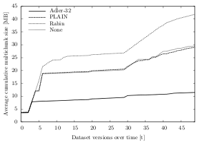 | 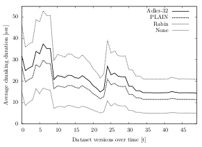 |
| Figure 6.8: Average cumulative multichunk size over time, compared by fingerprinting algorithm (dataset A) | Figure 6.9: Average chunking duration, clustered by fingerprinting algorithm (dataset B) |
The results of the experiment show that the Adler-32 fingerprinter outperforms the other algorithms in terms of chunking efficiency in all datasets. Over all test runs, the Adler-32 average temporal deduplication ratio is 14.7:1 (space reduction of 93.2%) – compared to a ratio of only 11.2:1 for the PLAIN algorithm (space reduction of 91.1%). With a ratio of 10.3:1 (space reduction of 90.3%), the Rabin algorithm performs the worst out of all four. In fact, its average temporal deduplication ratio is worse than the average of the fixed-size chunking algorithms (ratio of 10.8:1, space reduction of 90.7%).
Figure 6.8 illustrates the different chunking efficiency of the fingerprinting algorithms for dataset A. In the first run, all algorithms create multichunks of similar size (about 3.6 MB). After the data has been changed 50 times, however, the multichunks created by Adler-32 add up to only 11.4 MB, whereas the ones created by Rabin are almost four times as big (41.8 MB). Even though the multichunks created by PLAIN and the fixed-size algorithm are significantly smaller (about 29 MB), they are still 2.5 times bigger than the ones created using the Adler-32 fingerprinter.
For dataset C, Adler-32 creates about 25% smaller multichunks than the other algorithms: After 50 test runs, the average size of the multichunks created from dataset C is 245.5 MB (temporal deduplication ratio of 24.4:1, space reduction of 95.9%), whereas the output created by the other fingerprinters is larger than 325 MB. Compared to PLAIN, for instance, Adler-32 saves 80.6 MB of disk space. Compared to Rabin, it even saves 102.5 MB.
Looking at dataset B, the space savings are not as high as with the other datasets: The temporal deduplication ratio is 19.4:1 (space reduction of 94.8%) and the multichunk output is 1,462 MB – compared to 1,548 MB for PLAIN (deduplication ratio of 18.4:1, space reduction of 94.5%). Even though the space reduction after 50 dataset versions is not as high compared to the other datasets, it still saves 85.9 MB.
The CPU usage of the fingerprinters largely behaves as expected. With an average of 93.5%, Rabin has a higher average CPU usage than PLAIN with 92.4% and much higher than the fixed-size algorithms with 90%. Surprisingly, Adler-32 uses the most processor time (average CPU usage of 95.1%) – even though its algorithm is solely based on additions and shift-operations (as opposed to calculations based on irreducible polynomials in the Rabin fingerprinting algorithm).
In terms of chunking duration, the fixed-size algorithms are certainly faster than the variable-size algorithms based on TTTD (as shown in section 3.4.3.1). In fact, they take about half the time than the PLAIN algorithms and less than a third than the algorithms using the Rabin fingerprinter. Over all datasets and test runs, the average chunking duration for algorithms with fixed-offset chunking is 4.1 seconds, for PLAIN based algorithms it is 8.3 seconds, for Adler-32 based algorithms it is 10.0 seconds and for Rabin based algorithms it is 13.7 seconds.
Figure 6.9 shows the differences in the chunking duration over time for dataset B: Algorithms using Rabin as fingerprinting mechanism are significantly slower than algorithms using other or no fingerprinters. Rabin is on average about 9 seconds slower than PLAIN and Adler-32 and over 20 seconds behind the algorithms without fingerprinter (fixed). Totalling this extra time over 50 changesets, Adler-32 is about 7.5 minutes faster than Rabin, PLAIN about 11 minutes and fixed-size algorithms over 18 minutes.
6.4.3.3. Compression Algorithm
After a multichunk has been closed (because the target size is reached), it is further compressed using a compression algorithm. When analyzing the chunking efficiency in regard to what compression algorithm has been used, the results in all datasets show that Bzip2 produces the smallest multichunks, but at the same time has a higher CPU usage than the other options Gzip and None. While these results are consistent throughout all datasets, the difference between the compression algorithms is marginal.
Over all datasets and test runs, the Bzip2 algorithm creates an output that is about 2% smaller than the one created using Gzip and about 42% smaller than without the use of a compression algorithm. The average temporal deduplication ratio with Bzip2 is 13.06:1 (space reduction of 92.3%), whereas when using Gzip, the ratio is 12.6:1 (space reduction of 92.0%). Without any compression, the average temporal deduplication ratio is 9.6:1 (space reduction of 89.6%).
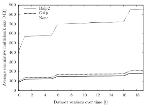 | 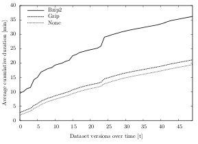 |
| Figure 6.10: Average cumulative multichunk size over time, clustered by compression algorithm (dataset D) | Figure 6.11: Average cumulative overall duration over time, clustered by compression algorithm (dataset B) |
For datasets A, B and C, the temporal deduplication ratio of Bzip2 and Gzip after 50 changes differs by only 0.3, i.e. the size of the generated multichunks is almost identical (max. 2% spread). Expressed in bytes, the Gzip/Bzip2 spread is only about 100 KB for dataset A (27.8 MB and 27.7 MB), 8 MB for dataset B (1,492 MB and 1,500 MB) and 6 MB for dataset C (300 MB and 294 MB).
For dataset D, the difference of the multichunk sizes between Gzip and Bzip2 is slightly higher (13% spread, about 24 MB), but very small compared to the spread between compression (Gzip/Bzip2) and no compression. Figure 6.10 illustrates these differences for dataset D over time: Starting in the first run, the algorithms with Gzip or Bzip2 compression create multichunks of under 100 MB, whereas the multichunks created by the algorithms without compression are about four times the size (412 MB). Over time, this 312 MB spread grows even bigger and the cumulative multichunk size of Gzip and Bzip2 add up to about 200 MB, compared to 855 MB for the no compression algorithms (655 MB spread).
In terms of CPU usage, the algorithms with Bzip2 use an average of 94%, while the ones using the Gzip algorithm use an average of 92.4%. Without compression, the CPU usage average over all datasets and test runs is 91.9%. While Bzip2 consumes the most processing time on average, the percentage is not constantly greater than the CPU usage numbers of Gzip and no compression. In fact, in dataset A and B, the algorithms without compression and the Gzip algorithms use more CPU than the Bzip2 algorithms.
Regarding the speed of the compression algorithms, Bzip2 is significantly slower than the other two compression options. With regard to all datasets and test runs, Bzip2 has an average overall per-run duration4 of 20.6 seconds, Gzip has a moderate speed (average 12.5 seconds) and not compressing the multichunks is the fastest method (11.5 seconds). Gzip is about 63% faster than Bzip2, not compressing is about 78% faster. The difference between Gzip and not compressing the multichunks is only about 8%.
Looking at dataset B in figure 6.11, for instance, the average cumulative overall duration using Bzip2 is much higher than for the options Gzip and None. In the first run, the algorithms using Gzip run less than 3 minutes, the ones without any compression only 2 minutes. The ones using Bzip2 as compression algorithm, however, run more than three times longer (9.5 minutes). This significant speed difference carries on throughout all test runs and leads to an overhead of about 15 minutes between Bzip2 and Gzip and about 17 minutes between Bzip2 and the no compression algorithms.
6.4.3.4. Chunk Size
The chunk size parameter defines the target size of the resulting chunks of the algorithm. Generally, smaller chunk sizes lead to a higher deduplication ratio, but require more CPU time.
Even though these statements match the results of the experiments, the impact of the parameter is not as high as expected. In fact, independent of the chosen chunk size (4 KB, 8 KB or 16 KB), the algorithm produces very similar results. Chunking efficiency, CPU usage and total chunking duration only differ marginally in their results.
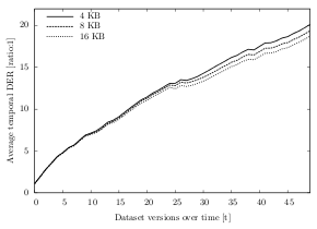 | 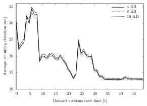 |
| Figure 6.12: Average temporal deduplication ratio over time, clustered by chunk size (dataset C) | Figure 6.13: Average chunking duration over time, clustered by the chunk size (dataset B) |
Over all datasets and test runs, the maximum temporal deduplication ratio for a chunk size of 4 KB is 26.7:1 (space reduction of 96.2%). For 8 KB, the best temporal deduplication ratio is 25.8:1 (space reduction of 96.1%) and for 16 KB it is 25.1:1 (space reduction of 96.0%).
Figure 6.12 shows the temporal deduplication ratio for dataset B. Independent of the chunk size, the average ratio develops almost identically for the three parameter values. After 50 snapshots of the dataset, the ratios are 20.1:1 (4 KB chunks), 19.3:1 (8 KB chunks) and 18.7:1 (16 KB chunks). Expressed in absolute values, the total cumulated multichunk size is 305.6 MB using 4 KB chunks, 316.7 MB using 8 KB chunks and 328.1 MB using 16 KB chunks. The results for other datasets have even closer ratios. The deduplication ratios of dataset B only differ by 0.16 (18.7:1 for 4 KB chunks, 18.6:1 for 8 KB chunks and 18.5:1 for 16 KB chunks) and of dataset A by only 0.10.
The average CPU usage, clustered by the three parameters, is very similar. With 4 KB chunks, the average CPU usage over all test runs is 95.1%, for 8 KB chunk size it is 94.9% and for 16 KB chunk size it is 95.5%. In fact, for datasets B and C, the mean deviation of the CPU usage per test run is only 0.5% and 0.4%, respectively. Only dataset A shows significant differences in the CPU usage: Its average deviation is 7.7%, its median deviation 4.7%.
Similar to the CPU usage, the chunking duration is also hardly affected by the size of the created chunks. Independent of the parameter value, the overall chunking duration is very similar. As table 6.2 shows, the average chunking duration per test run and dataset are completely decoupled from the chunk size. Even for dataset B, for which the cumulated chunking duration is over 15 minutes, the time difference after the last run is less than one minute. For the smaller datasets A and C, the average duration is almost identical (for A about 10 seconds, for C about 3 minutes, 38 seconds).
| Max. Deduplication Ratio | Avg. Chunking Duration | |||||
| Chunk Size | Dataset A | Dataset B | Dataset C | Dataset A | Dataset B | Dataset C |
| 4 KB | 26.33:1 | 20.17:1 | 26.76:1 | 10 sec | 15:29 min | 3:38 min |
| 8 KB | 25.68:1 | 20.00:1 | 25.81:1 | 10 sec | 15:52 min | 3:38 min |
| 16 KB | 24.47:1 | 19.77:1 | 25.15:1 | 9 sec | 15:11 min | 3:37 min |
Table 6.2: Maximum temporal deduplication ratio per dataset (left) and average chunking duration per dataset (right), both clustered by chunk size.
Figure 6.13 illustrates the average chunking durations for dataset B, clustered by the chunk size: The more files are changed/updated/new in between the indexing runs, the longer it takes to complete the chunking process. However, while the duration differs significantly in each run (about 35 seconds in the sixth run vs. about 12 seconds for the last run), it only marginally varies for the different chunk sizes (average deviation of 0.5 seconds).
6.4.3.5. Write Pause
The write pause parameter defines the number of milliseconds the chunking algorithm sleeps after each multichunk. The parameter is meant to artificially slow down the chunking time in order to lower the average CPU usage.
The results of the experiments show that the algorithms without a sleep time (0 ms) have an 11% higher average CPU usage – compared to the ones with a 30 ms write pause in between the multichunks. On average, the 0 ms-algorithms use 98.8% CPU, whereas the 30 ms-algorithms use 87.8%.
Figure 6.14 shows the effects of the write pause parameter during the chunking and indexing process of dataset B. Without sleep time, all of the values are above 89% and the average CPU usage is 96.7% – i.e. the CPU is always stressed. With a short write pause in between the multichunks, the average is reduced to 90.3%.
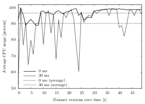 | 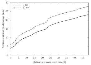 |
| Figure 6.14: Average CPU usage over time, clustered by the write pause (dataset B). | Figure 6.15: Cumulative chunking duration over time, clustered by write pause (dataset B). |
While the parameter has a positive effect on the CPU usage, it lengthens the overall chunking duration. On average, 30 ms-algorithms run 19.8% longer than the ones without pause. For the datasets in the experiments, this longer duration ranges from a few seconds for small datasets (additional 6 seconds for dataset A) to many minutes for larger ones (additional 5 minutes for dataset B). Broken down to the chunking process of a single snapshot, the additional time is rather small: 0.12 seconds for dataset A, 5.6 seconds for dataset B and 1.3 seconds for dataset C.
Figure 6.15 illustrates the cumulative duration5 while chunking dataset B. Since the underlying calculations and algorithms are identical, the two curves develop similarly – only with a vertical shift. In fact, the correlation of both curves is 0.99.
The write pause parameter has no impact on the chunking efficiency, i.e. on the temporal deduplication ratio, because it does not alter the algorithm itself, but rather slows it down.
6.4.3.6. Multichunk Size
The multichunk size parameter controls the minimum size of the resulting multichunks. Rather than influencing the chunking efficiency, it aims at maximizing the upload bandwidth and minimizing the upload duration (see experiment 2 in section 6.5). Even though the impact of the parameter on the chunking efficiency is small, it must be part of the analysis.
The results of the experiments show that the average DER with a minimum multichunk size of 250 KB is slightly higher than when 125 KB multichunks are created. Over all datasets and test runs, the average temporal deduplication ratio is 11.8:1 (space reduction of 91.5%) for algorithms with 250 KB multichunk containers and 11.7:1 (space reduction of 91.4%) for algorithms with 125 KB multichunks. The difference in the deduplication ratio is below 0.1 for datasets A, B and C, but as high as 0.6 for dataset D.
In terms of CPU usage, algorithms using 125 KB multichunks use less CPU, because they have about double the amount of write pauses in the chunking process. 125 KB algorithms use an average of 91.7% CPU, whereas algorithms creating 250 KB multichunks use 93.9% CPU.
The additional write pauses in the 125 KB algorithms also affect the overall duration. On average, algorithms creating 250 KB chunks are about 8% faster than algorithms creating 125 KB chunks. The overall average duration per run for the 125 KB option is 15.4 seconds, whereas the overall average for the 250 KB option is 14.3 seconds.
Looking at dataset C, for instance, the mean difference in the initial run is only about 9 seconds (53 seconds for 250 KB algorithms, 62 seconds for 125 KB algorithms). Over time, i.e. after chunking and indexing 50 versions, the average cumulated difference is still only 21 seconds (363 seconds for 125 KB algorithms, 342 seconds for 250 KB algorithms).
6.4.3.7. Overall Configuration
Having analyzed the individual parameters and their behavior in the experiment, this section focuses on the overall configuration of these parameters. In order to finally choose a suitable configuration for Syncany, this section is of particular importance. While the previous sections focused on only one parameter at a time, this section is able to weigh the parameters against each other and make statements about individual parameters in the overall context.
Deduplication ratio: Table 6.3 gives an excerpt of the best overall parameter configuration with respect to the average deduplication ratio (full table in appendix D). The results of the experiment confirm the expectations to a large extent on all of the four datasets.
| Rank | Algorithm Configuration | A | B | C | D | Average | |
| 1 | Custom-250-*/TTTD-4-Adler32/Bzip2-Cipher | 15.35 | 12.88 | 15.43 | 32.67 | 16.68 | |
| 2 | Custom-125-*/TTTD-4-Adler32/Bzip2-Cipher | 15.33 | 12.84 | 15.40 | 30.92 | 16.45 | |
| 3 | Custom-250-*/TTTD-8-Adler32/Bzip2-Cipher | 15.13 | 12.80 | 15.00 | 30.56 | 16.22 | |
| 4 | Custom-250-*/TTTD-4-Adler32/Gzip-Cipher | 15.37 | 12.82 | 15.37 | 28.31 | 16.14 | |
| 5 | Custom-125-*/TTTD-4-Adler32/Gzip-Cipher | 15.39 | 12.82 | 15.38 | 27.99 | 16.11 | |
| 6 | Custom-125-*/TTTD-8-Adler32/Bzip2-Cipher | 15.12 | 12.75 | 14.96 | 29.00 | 16.01 | |
| 7 | Custom-250-*/TTTD-16-Adler32/Bzip2-Cipher | 14.55 | 12.67 | 14.68 | 28.74 | 15.71 | |
| 8 | Custom-250-*/TTTD-8-Adler32/Gzip-Cipher | 15.16 | 12.73 | 14.94 | 26.37 | 15.70 | |
| 9 | Custom-125-*/TTTD-8-Adler32/Gzip-Cipher | 15.17 | 12.73 | 14.94 | 26.11 | 15.67 | |
| 10 | Custom-125-*/TTTD-16-Adler32/Bzip2-Cipher | 14.53 | 12.63 | 14.66 | 27.29 | 15.51 | |
| ... | ... | ... | ... | ... | ... | ... | |
| 67 | Custom-250-*/TTTD-16-Rabin/Cipher | 6.00 | 11.23 | 9.31 | 5.53 | 8.46 | |
| 68 | Custom-125-*/TTTD-16-Rabin/Cipher | 6.00 | 11.23 | 9.31 | 5.53 | 8.46 | |
| 69 | Custom-250-*/TTTD-8-Rabin/Cipher | 5.26 | 11.24 | 9.81 | 5.67 | 8.40 | |
| 70 | Custom-125-*/TTTD-8-Rabin/Cipher | 5.26 | 11.24 | 9.81 | 5.67 | 8.40 | |
| 71 | Custom-250-*/TTTD-4-Rabin/Cipher | 3.99 | 11.27 | 9.74 | 5.79 | 8.03 | |
| 72 | Custom-125-*/TTTD-4-Rabin/Cipher | 3.98 | 11.27 | 9.74 | 5.79 | 8.03 |
Table 6.3: Average temporal deduplication ratio over all datasets (as ratio:1), clustered by algorithm configuration and sorted by the average. The full list can be found in appendix D.
With regard to the deduplication ratio and the derived space reduction percentage, the chunking method and the fingerprinting algorithm have the strongest influence on the result: In terms of the chunking method, the variable-size algorithm TTTD is used in all of the top third algorithm configurations (first 24). However, it is also used in 18 of the worst 24 algorithms. 6
Looking at the fingerprinters, the Adler-32 algorithm has proven most effective for all of the analyzed datasets. In the overall ranking, 16 out of 18 Adler-32 algorithms appear in the first third of the table and all of them are present in the first half. The other fingerprinters are distributed over the whole ranking, with PLAIN mostly in the mid-range and Rabin performing worst. In fact, none of the top 24 algorithms use the Rabin fingerprinter and only two of the first half do.
Besides chunker and fingerprinter, the compression algorithm is of particular relevance in terms of deduplication ratio: Over 80% of the best 24 algorithms use compression – equally divided between Gzip and Bzip2 (10 configurations each). Most of the algorithms without compression (18 of 24) reside at the end of the table, with the lowest average temporal deduplication ratio.
Even though the chunk size was expected to have a high influence on the chunking efficiency, the impact is small compared to the other parameters. For the chunk sizes 4 KB and 8 KB, about 83% of the algorithm configurations are in the top third of the list (41.6% each) and about 17% are algorithms with 16 KB chunks. Particularly the two options 4 KB and 8 KB have a similar distribution in the list and do not seem to differ much with regard to the deduplication ratio. The 16 KB option, however, differs in its impact on the DER: About 70% of the algorithms in the bottom half of the list use 16 KB chunks.
The multichunk size is by far the parameter with the least relevance to the deduplication ratio: 125 KB and 250 KB algorithm configurations are equally distributed amongst the ranking. 19 of the 36 algorithms with 250 KB multichunks are in the upper half of the list, 17 in the bottom half. Conversely, 17 of 36 algorithms with 125 KB chunks are in the top half of the table, 19 in the bottom half. In fact, the difference is so marginal that the 125 KB and 250 KB configurations with otherwise identical parameters are often very close together in the list (if not right behind each other).
Looking at the absolute ratios in table 6.3, the difference among the configurations is quite big: While the best algorithm configuration Custom-250-*/TTTD-4-Adler32/Bzip2-Cipher has an average deduplication ratio of 16.7:1 (space reduction of 94%), the worst configuration Custom-125-*/TTTD-4-Rabin/Cipher only reaches an average of 8:1 (space reduction of 87.5%).
When looking at the differences between the datasets, the deduplication ratio differs significantly: The ratio reaches an average of 32.6:1 (space reduction of 96.9%) in dataset D for the best configuration and less than half for dataset C (ratio of 12.9:1, space reduction of 92.2%). For the worst configuration, the best average ratio is reached by dataset B with 11.3:1 (space reduction of 92.1%) and the worst ratio by dataset A (ratio of 4:1, space reduction of 74.8%). Depending on the data in the dataset, the spread between the best and the worst configuration can be higher or lower. While the best/worst-spread in dataset B is only 1.6 (12.9:1 and 11.3:1), the ratio difference for dataset D is 26.9 (32.7:1 and 5.8:1).
Total duration: The overall duration behaves almost reverse to the temporal deduplication ratio. Many well-performing parameters in terms of chunking efficiency slow down the overall chunking process. Table 6.4 gives an excerpt of the ranking with regard to the overall per-run duration (full table in appendix E).
| Rank | Algorithm Configuration | A | B | C | D | Average |
| 1 | Custom-250-0/Fixed-8/Cipher | 0.10 | 9.09 | 1.70 | 12.92 | 4.72 |
| 2 | Custom-250-0/Fixed-16/Cipher | 0.10 | 8.60 | 1.64 | 14.58 | 4.75 |
| 3 | Custom-125-0/Fixed-16/Cipher | 0.09 | 10.62 | 1.64 | 15.16 | 5.42 |
| 4 | Custom-250-0/Fixed-4/Cipher | 0.10 | 10.88 | 1.88 | 16.82 | 5.76 |
| 5 | Custom-250-0/Fixed-16/Gzip-Cipher | 0.14 | 11.14 | 2.22 | 15.56 | 5.80 |
| 6 | Custom-125-0/Fixed-8/Cipher | 0.10 | 11.99 | 1.71 | 15.13 | 5.84 |
| 7 | Custom-125-0/Fixed-4/Cipher | 0.10 | 10.84 | 1.96 | 17.72 | 5.88 |
| 8 | Custom-125-0/Fixed-16/Gzip-Cipher | 0.14 | 11.00 | 2.20 | 16.91 | 5.91 |
| 9 | Custom-250-0/Fixed-8/Gzip-Cipher | 0.14 | 11.66 | 2.28 | 15.89 | 6.01 |
| 10 | Custom-125-0/Fixed-8/Gzip-Cipher | 0.14 | 11.52 | 2.28 | 17.41 | 6.15 |
| ... | ... | ... | ... | ... | ... | ... |
| 139 | Custom-250-30/TTTD-16-Rabin/Bzip2-Cipher | 0.90 | 54.34 | 13.69 | 46.29 | 25.72 |
| 140 | Custom-250-30/TTTD-8-Rabin/Bzip2-Cipher | 1.02 | 54.32 | 13.31 | 47.99 | 25.84 |
| 141 | Custom-250-30/TTTD-4-Rabin/Bzip2-Cipher | 1.13 | 56.06 | 13.27 | 48.94 | 26.48 |
| 142 | Custom-125-30/TTTD-16-Rabin/Bzip2-Cipher | 0.99 | 57.88 | 14.60 | 53.20 | 27.87 |
| 143 | Custom-125-30/TTTD-8-Rabin/Bzip2-Cipher | 1.11 | 58.72 | 14.24 | 54.79 | 28.23 |
| 144 | Custom-125-30/TTTD-4-Rabin/Bzip2-Cipher | 1.26 | 60.13 | 14.27 | 56.16 | 28.86 |
Table 6.4: Average overall per-run duration over all datasets in seconds, clustered by algorithm configuration and sorted by the average. The full list can be found in appendix E.
As it is visible from the table, the factor with the gratest influence on the overall speed of the algorithm is the chunking method: While TTTD produces the better DER results, the fixed-size chunking algorithms are significantly faster. Overall, all of the 17 top algorithm configurations use a fixed-size chunker instead of a variable-size chunker. About 66% of the fixed-size configurations are in the top third of the ranking and over 72% in the first half. Conversely, less than 23% of the TTTD-based algorithms are in the list of the best 48 configurations.
With the values of this experiment, the second most important factor is the write pause: The top 12 of all algorithm configurations have no write pause in between the multichunks, i.e. the write pause parameter is set to 0 ms. Overall, about 66% of the algorithms in the first third have no write pause. On the contrary, 30 of the 48 last configurations have the parameter set to 30 ms.
Apart from the chunking method, compression is the parameter with the second highest impact: Depending on the compression method, algorithms can be signficantly slower. For this ranking, 77% of the algorithms without compression can be found in the first half of the list. The Bzip2 algorithm in particular is not used in any of the first 48 configurations and in only two of the first 72 algorithms. In fact, the last 19 configurations use the Bzip2 algorithm to compress their multichunks. Compared to that, Gzip is much more prominent in the top part of the list: About 44% of the upper half algorithms use the Gzip compression.
When TTTD is used, the fingerprinting method is an important factor to influence the speed. In the experiments, the Rabin method has proven to be by far the slowest: In the first third of all configurations, none of the algorithms used Rabin as fingerprinter and only two of the first half did. Conversely, about 94% of all algorithms using Rabin can be found in the bottom half of the list – 12 of them on the ranks 133–144. Compared to that, the other fingerprinters do not have that much influence on the speed. PLAIN occurs in 15 of the first 48 algorithms, Adler-32 in only 9.
The last two parameters, multichunk size and chunk size, have no visible impact on the overall duration at all. The algorithm configurations with the multichunk sizes 125 KB and 250 KB distribute evenly in the ranking: 45% of 125 KB algorithms in the top half, 54% in the bottom half – and vice versa for the 250 KB algorithms. For the chunk sizes 4 KB, 8 KB and 16 KB, the situation is similar. For all of them, there are around 33% of each configuration in the first third/half.
CPU usage: The average processor usage is in many properties similar to the overall duration. As with the duration, some DER-improving parameters increase the CPU percentage. Table 6.5 shows an excerpt of the best algorithm configurations with regard to the CPU usage. Since the amount of data in dataset A was very small and a test run was often faster than a second, the CPU measurements are not reliable. Average values and ranking do not include the measurements of dataset A.
| Rank | Algorithm Configuration | A | B | C | D | Average |
| 1 | Custom-125-30/Fixed-16/Cipher | 67.12 | 78.58 | 65.28 | 54.30 | 66.05 |
| 2 | Custom-125-30/Fixed-8/Cipher | 75.44 | 80.86 | 66.14 | 53.55 | 66.85 |
| 3 | Custom-125-30/Fixed-16/Gzip-Cipher | 70.36 | 81.92 | 70.02 | 52.50 | 68.15 |
| 4 | Custom-125-30/Fixed-4/Cipher | 72.28 | 82.70 | 67.84 | 57.45 | 69.33 |
| 5 | Custom-125-30/Fixed-8/Gzip-Cipher | 79.82 | 83.26 | 70.56 | 55.60 | 69.81 |
| 6 | Custom-125-30/Fixed-4/Gzip-Cipher | 76.42 | 84.04 | 71.88 | 56.85 | 70.92 |
| 7 | Custom-250-30/Fixed-8/Cipher | 85.22 | 85.72 | 76.60 | 54.15 | 72.16 |
| 8 | Custom-250-30/Fixed-16/Cipher | 70.88 | 84.02 | 76.20 | 58.20 | 72.81 |
| 9 | Custom-250-30/Fixed-4/Cipher | 78.50 | 87.50 | 77.90 | 58.90 | 74.77 |
| 10 | Custom-250-30/Fixed-16/Gzip-Cipher | 74.96 | 86.92 | 80.18 | 59.05 | 75.38 |
| ... | ... | ... | ... | ... | ... | ... |
| 139 | Custom-125-0/TTTD-16-Rabin/Gzip-Cipher | 105.90 | 99.02 | 99.34 | 85.60 | 94.65 |
| 140 | Custom-125-0/TTTD-8-Rabin/Gzip-Cipher | 103.82 | 99.52 | 99.40 | 85.05 | 94.66 |
| 141 | Custom-250-0/TTTD-16-Rabin/Gzip-Cipher | 103.80 | 99.08 | 99.24 | 86.05 | 94.79 |
| 142 | Custom-250-0/TTTD-8-Rabin/Cipher | 106.78 | 99.04 | 99.14 | 87.15 | 95.11 |
| 143 | Custom-250-0/TTTD-4-Rabin/Cipher | 111.20 | 97.98 | 99.40 | 88.35 | 95.24 |
| 144 | Custom-250-0/TTTD-8-Rabin/Gzip-Cipher | 103.24 | 99.60 | 99.22 | 87.70 | 95.51 |
Table 6.5: Average CPU usage in percent, clustered by algorithm configuration and sorted by the average. Due to unreliable measurements in dataset A, its values are ignored in ranking and average. The full list can be found in appendix F.
The greatest influence on the average CPU usage is the write pause parameter: Most of the algorithm configurations with the lowest average CPU usage have set the parameter to 30 ms. Out of the 48 top configurations in the ranking, 44 are 30 ms-configurations. Conversely, only 4 of the 0 ms-configurations are in the top third and only 14 in the top half.
The parameter with the second greatest impact on the processor usage is the chunking method: The top 13 algorithms in the ranking use a fixed-size chunker and nearly 90% of all fixed-size algorithms can be found in the top half of the ranking.
Apart from the chunking method and the write pause, the fingerprinting method has a great impact as well. In particular, algorithms using the Rabin fingerprinting method have a rather high CPU usage compared to other fingerprinters. In fact, 21 of the 36 algorithms using Rabin can be found in the bottom third of the list – 12 of them even on the last positions.
The impact of the multichunk size is not insignificant: 30 out of the 72 algorithms with 125 KB multichunks are in the top third of the ranking, whereas only 18 of the 250 KB algorithms appear in the table. That is about 63% of the first third are algorithms creating 125 KB multichunks.
The other parameters, namely chunk size and compression, are only marginally relevant in the overall context: In terms of compression, not compressing has slight advantages for the overall configuration. About 58% of the non-compressing algorithms are in the top half of the ranking, whereas over 53% of the algorithms using compression are in the bottom half. The chunk size has even less impact on the overall configuration. All algorithms with 4 KB, 8 KB and 16 KB chunks are equally distributed in the ranking, with about 33% of each in the first third/half.
| Lowest CPU | Lowest Duration | Highest DER | |
| Chunking Algorithm | Fixed | Fixed | TTTD |
| Fingerprinting Algorithm | None | None | Adler-32 |
| Compression Algorithm | None | None | Bzip2 |
| Chunk Size | & 16 KB | 16 KB | 4 KB |
| Write Pause | 30 ms | 0 ms | indiff. |
| Multichunk Size | 125 KB | 250 KB | 250 KB |
Table 6.6: Best configuration parameters with regard to the respective aims of minimizing the CPU usage, minimizing the total duration as well as maximizing the temporal deduplication ratio.
Table 6.6 illustrates the best values with regard to the respective goals that have been derived from the results of the experiments.
6.4.4. Discussion
After analyzing the results of the experiments, this section aims at interpreting and discussing these results in the scope of Syncany. In particular, its goal is to find a suitable overall algorithm configuration – with regard to Syncany’s environment and requirements.
In the typical Syncany use case, the application runs in the background and the user is not supposed to be disturbed by it (low CPU usage). In some cases, the user’s goal is to simply backup some data (duration marginally relevant). In other cases, it is to share files with other users as quickly as possible (duration very relevant). Similarly, sometimes the remote storage is paid per GB, in other cases the storage is limited in size (high DER desired).
The experiment above targeted these goals and tried to optimize the generic deduplication algorithm by changing the input parameters. As the results show, many of the parameters perform quite well in one or two of these goals, but not in all of them. In fact, many of the DER-improving parameters such as Adler-32 or Bzip2 perform badly in terms of overall duration or CPU usage. Vice versa, parameters with better speed and CPU performance such as the fixed-size chunking method perform worse in terms of space savings.
With regard to the goal of Syncany as an end-user application, one of the most basic requirements is to make its usage easy and non-disruptive to other applications. It must hence be the first priority to reduce the CPU usage and hide the deduplication process from end-users. Chunking efficiency and overall duration must be considered secondary – at least for this case. 7
Taking the reduction of CPU usage as the primary goal, all of the algorithm configurations analyzed in the experiment show a rather weak performance: Most of the configurations with a relatively high average deduplication ratio have CPU averages around 90%. For a background end-user application, this value is unacceptable. Instead, a much lower average should be targeted in the selection of a suitable algorithm. Values around 20–30% are acceptable, given that the application only needs resources for a limited time.
While the results of the experiments help identifying parameters with extremely bad CPU impact, they do not clearly state a winner in terms of overall configuration. Even the best configurations have far higher averages than desired. In fact, the high CPU usage indicates that other means are necessary to limit processor usage.
The write pause parameter, for instance, is intended to fulfill this exact purpose, but has not succeeded to reliably control processor usage limits: While the parameter can lower the average CPU usage, it does not allow setting a maximum percentage or take the differences of the underlying data into account. Due to the many small text files in dataset D, for instance, the average processor usage is much lower than in dataset C. Using the same algorithm, the resulting difference in the CPU usage is often over 20%.
Instead of having a single fixed write pause parameter such as 30 ms, an effective algorithm should dynamically adjust this parameter depending on the measured CPU usage. An algorithm could, for instance, increase the write pause up to 100 ms or 150 ms, if the CPU is stressed and lower it when the percentage is below the maximum.
Having the other goals in mind, some of the other parameters must be tolerated as-is despite their bad CPU performance. Variable-size chunking methods and some of the corresponding fingerprinting algorithms, for instance, have a rather high impact on the temporal deduplication ratio. Even though their average processor usage is high in the experiments, a dynamic write pause parameter could artificially slow down the algorithm to decrease the processor usage. In fact, since all configurations can be slowed down, it makes sense to only eliminate the parameter values that evidently cause a significantly higher CPU usage.
The most noticeable parameter is the Rabin fingerprinting algorithm: As already discussed in section 6.4.3.2 (and also visible in tables 6.5 and F.1), algorithms using Rabin and Adler-32 have a higher average CPU usage than other algorithms. However, while Adler-32 has a superior average deduplication ratio and overall runtime, Rabin performs quite bad in all measures – and is hence not suitable as potential parameter.
The second parameter with obvious negative influence on the average CPU usage is the compression algorithm Bzip2. Compared to Gzip, it uses more CPU cycles and appears in many of the worst performing algorithm configurations. Additionally, it performs exceptionally bad in terms of overall duration. In particular when combining Bzip2 with a potentially higher (or dynamic) write pause parameter, the algorithm would run slower by the orders of magnitude. It, too, is not suitable as a potential parameter for Syncany.
Assuming that the write pause parameter can counteract the potentially bad CPU impact of the other parameters, the second most important factor is the efficiency of the chunking algorithm: Given that remote storage often costs money, minimizing the data to store also reduces the total cost of storage. Additionally, reducing the overall amount of data also reduces the time to upload/download it from the storage and thereby accelerates the overall time of synchronization between two Syncany clients.
As already discovered in section 6.4.3.7, the parameter with the greatest positive influence on the deduplication ratio is the Adler-32 fingerprinting algorithm. It performs well for all datasets and has – despite the relatively high processor usage – no negative properties. In fact, compared to the other fingerprinters, the achieved space savings due to Adler-32 are remarkably high and cannot compare to the other fingerprinting mechanisms.
Given the outstanding performance of the algorithm, it makes sense to choose Adler-32 as the fingerprinter of choice for Syncany. And since that implies a variable-size chunker, TTTD is by definition the most suitable chunking method. Conversely, that disqualifies the fixed-size chunker and the PLAIN fingerprinter as primary choice for Syncany’s deduplication algorithm.
| Chosen Value | Explanation | |
| Chunker | TTTD | Variable-sized chunking allows for higher space savings than fixed-size chunking. |
| Fingerprinter | Adler-32 | Adler-32 outperforms the other options in terms of deduplication. Rabin performs bad in all measures. |
| Compression | Gzip | Bzip2 is too slow and the no compression option performs bad on pure text files. |
| Chunk Size | 4 KB | The chunk size is almost indifferent in regard to all measures. 4 KB chunks deliver better deduplication results. |
| Write Pause | ≥ 30 ms | The 30 ms option reduces CPU usage, but not enough for Syncany. Dynamic write pauses are desirable. |
| Multichunk Size | 250 KB | The analyzed values are largely indifferent. The 250 KB variant has a higher DER. |
Table 6.7: Chosen values for Syncany based on the results of experiment 1.
From the perspective of the deduplication ratio, the last parameter with significant impact on the space savings is the no compression parameter. While Bzip2 is already disqualified due to high CPU usage and extremely long overall runtime, both Gzip and no compression are still viable options. However, while Gzip performs acceptable with regard to reducing the size of the resulting multichunks, not using compression has shown to be very ineffective. As shown in section 6.4.3.3, it performs bad on all datasets, but in particular on plain text files (dataset D). For Syncany, this fact eliminates no compression as a viable option.
The two left over parameters chunk size and multichunk size have hardly any impact on any of the measures. All parameter values share similar CPU usage percentages, average duration values and average temporal deduplication ratios. With regard to these findings, the best parameter for Syncany in the respective category is the one with the highest DER – even though its difference to the other values is small. For the chunk size, the best value in that regard is 4 KB (as opposed to 8 KB and 16 KB). For the multichunk size parameter, this value is 250 KB.
Table 6.7 shows the values chosen for Syncany and summarizes the reasoning behind the decision. In the syntax of this thesis, the chosen overall algorithm configuration for Syncany is Custom-250-30/TTTD-4-Adler32/Gzip-Cipher.
In the rankings (as described in section 6.4.3.7), this algorithm ranks at 4 of 72 in the DER ranking (appendix D), at 64 of 144 in the duration ranking (appendix E) and at 62 of 144 in the CPU ranking (appendix F).
While the deduplication ranking is undoubtably very good, the other two only place the algorithm at the end of the top half. Even though that seems bad, it must be examined with care. Most of the top algorithms in the duration ranking are 0 ms-algorithms and/or Fixed-algorithms. After eliminating these options, it ranks in the top third. Similarly, the rank in the CPU table is only partially relevant, given that the CPU usage can be regulated with a higher (or dynamic) write pause parameter.
Overall, the chosen algorithm is a good trade-off between space reduction, CPU usage and runtime.
6.5. Experiment 2: Upload Bandwidth
Experiment 1 measured the chunking efficiency and tried to minimize the total size of the created chunks and multichunks. The goal of the experiment was to reduce the data that has to be transferred to the remote storage. While chunking efficiency is an important factor to reduce the upload bandwidth consumption, it is not the only relevant determinant. As discussed in chapter 5.1.3, the number of required upload requests can have a large impact on the request overhead and the upload duration.
The goal of this experiment is to prove that the multichunk concept maximizes the overall upload bandwidth independent of the storage type. In particular, it aims at reducing the overall upload duration (and thereby maximize the total upload bandwidth). It furthermore analyzes the upload behavior with regard to different types of storage.
The experiment is based on the results of the previous experiment and measures the upload duration and upload bandwidth with regard to the chosen chunk size and storage type.
6.5.1. Experiment Setup
The experiment runs the Java application UploadTests using the results from experiment 1: As input, it takes the average chunk sizes for each test run and dataset (for the target chunk sizes 4 KB, 8 KB and 16 KB and the multichunk sizes 125 KB and 250 KB) as well as the total size of the created multichunks per run (data to upload each run).
Using these average chunk sizes, it creates dummy chunks (random data) and uploads these chunks as files to the remote storage (FTP, S3 and IMAP). It measures the upload time and then derives the upload bandwidth. In order to cancel out interferences and factor in request latencies, it uploads each chunk multiple times and only stores the average duration.
For each dataset version, the application records the bytes uploaded, the upload duration and the derived upload bandwidth in KB/s. It furthermore derives the total upload duration as if the whole multichunk data were to be uploaded (linearly scaled).
6.5.2. Expectations
The multichunk concept aims at reducing the latency produced by uploading too many small files to a remote storage. By grouping chunks into multichunks, the number of upload requests is reduced. This reduction is expected to lower the total request overhead from the individual upload requests, reduce latency and increase the total upload bandwidth. Independent of the type of remote storage storage, the size of the uploaded payload is expected to directly influence the upload speed.
In particular, using smaller chunk sizes (4 KB, 8 KB and 16 KB) is expected to result in a significantly lower upload bandwidth than using larger chunk sizes (125 KB and 250 KB). That is using small chunks, the total upload time is expected to be higher than if multichunks are used.
Furthermore, it is expected that the type of storage has a direct influence on the average absolute upload speed, but not on the relative speed amongst the different chunk sizes. IMAP, for instance is expected to have a significantly lower average upload bandwidth than FTP or S3, because the payload is encoded using Base64. It is, however, not expected to behave differently than other storage types with respect to the chunk size.
6.5.3. Results
The experiment uploaded 514.1 MB to three different types of storage (FTP, S3 and IMAP). Overall, 20,910 chunks of different sizes were uploaded in the total duration of almost four hours.
The following sections present the results of the upload experiment. The analysis first looks at the size of the uploaded chunks in order to verify the multichunk concept and then identifies differences in the upload times between different storage types.
6.5.3.1. Chunk Size
The upload bandwidth is measured by dividing the number of uploaded bytes by the upload duration. In Syncany, a higher bandwidth is desirable, because it minimizes the time it takes to upload chunks and metadata. It thereby minimizes the time for clients to synchronize changes to the repository.
The results of this experiment show that the upload bandwidth largely behaves as expected: Over all datasets and storage types, the average upload bandwidth using 4 KB chunks is only about 21.2 KB/s, whereas the bandwidth using 250 KB chunks is about 60.5 KB/s. The upload speed of using the other chunk sizes lies in between those values: Using 8 KB chunks, the speed is about 31.1 KB/s, using 16 KB chunks, the speed is about 41.3 KB/s and using 125 KB chunks, the speed is about 57.0 KB/s.
Looking at dataset D in figure 6.16, for instance, the upload bandwidth spread can be observed over time: While the speed stays near 55 KB/s when using 125 KB chunks and around 65 KB/s for 250 KB chunks, the bandwidth never reaches 30 KB/s when 8 KB chunks are used and not even 20 KB/s when 4 KB chunks are used.
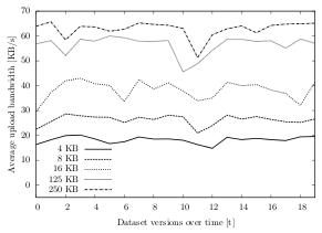 | 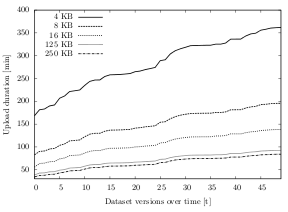 |
| Figure 6.16: Average upload bandwidth over time, clustered by chunk size (dataset D). | Figure 6.17: Cumulative average upload duration over time, clustered by chunk size (dataset C). |
Since the upload bandwidth is derived from the upload duration, its value behaves accordingly. On average, using 250 KB chunks is 4.4 times faster than using 4 KB chunks, about 2.8 times faster than using 8 KB chunks and about 1.8 times faster than using 16 KB chunks. The upload duration difference between 250 KB and 125 KB chunks is marginal: Using 250 KB chunks is about 13% faster than using 125 KB chunks. When excluding IMAP, this difference is even lower (7%).
Figure 6.17 shows these results for dataset C over time. With an initial upload duration of about 168 minutes using 4 KB chunks, compared to only 34 minutes when using 250 KB chunks, the 4 KB option is almost five times slower (134 minutes). This spread grows over time to a difference of over 4.5 hours (84 minutes using 250 KB chunks, 361 minutes using 4 KB chunks). While the spread from the 250 KB option to the 8 KB and 16 KB options is not as large as to the 4 KB option, it is significantly larger than between the 125 KB and 250 KB: Even after 50 uploads, the average cumulated 125/250 KB difference is less than 9 minutes, whereas the 16/250 KB spread is about 54 minutes.
6.5.3.2. Storage Type
The remote storage is the location at which the chunks or multichunks are stored. Depending on the underlying application layer protocol, chunks are transferred differently and the average upload bandwidth differs.
The results of the experiment show that the average upload bandwidth strongly depends on the storage type: Out of the three protocols within this experiment, the one with the highest average upload bandwidth is FTP with 54.1 KB/s, followed by the REST-based Amazon S3 with 49.1 KB/s and the e-mail mailbox protocol IMAP with only 23.6 KB/s (cf. figure 6.19).
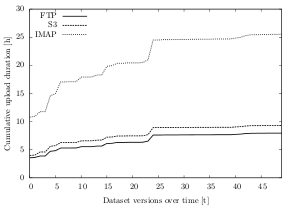 | 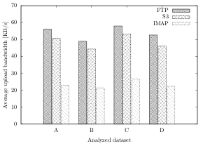 |
| Figure 6.18: Average cumulative upload duration over time, clustered by storage type (dataset B). | Figure 6.19: Average upload bandwidths, clustered by dataset and storage type (all datasets). |
While the bandwidth differs in its absolute values, the relative difference between the protocol speeds is very similar: FTP, for instance, is around 10% faster than Amazon S3 (± 2% in each dataset) and about 2.3 times faster than IMAP (± 3% in each dataset).
Figure 6.18 illustrates these different upload durations for dataset B: While the initial upload using FTP takes on average 3.5 hours and less than four hours using Amazon S3, storing the same amount of data in an IMAP mailbox takes over 10 hours. Over time, the spread grows to about 81 minutes between FTP and S3 (7.9 hours for FTP, 9.3 hours for S3) and to over 17 hours between FTP and IMAP (25.5 hours for IMAP).
6.5.4. Discussion
Having seen the results of the experiment, the multichunk concept has proven very effective to maximize the overall upload bandwidth. Independent of the underlying storage type, combining smaller chunks reduces the upload time and eliminates wait times. Due to a reduction of upload requests, the protocol-dependent latencies are minimized. For instance, instead of having 100 upload requests using 4 KB chunks, two requests with 250 KB multichunks are sufficient. The experiment has shown that the concept works regardless of the storage and independent of the dataset.
For Syncany, this method is valuable in two ways. First, it reduces the overall synchronization time between two or more Syncany clients. By increasing the upload speed, clients can publish their file changes faster and thereby enable a faster exchange of metadata and chunks. Second, it mitigates the effects of the different storage types. While the concept is not able to converge the speed of all protocols to the client’s maximum upload speed, it shifts the focus from the protocol-dependent request overhead to the speed of the actual upload connection.
Especially when looking at Syncany’s minimal storage interface (as described in chapter 4.5.4), decoupling from the specifics of the storage protocols reduces more of the protocol’s peculiarities. With protocols as different as Amazon S3 and IMAP, increasing the chunk size adds an extra layer of abstraction to this interface. Instead of having to deal with heavy-weight request headers or a high number of small requests in each Syncany plug-in, they behave alike even if the protocol differs significantly.
The overall algorithm configuration in experiment 1 includes 250 KB multichunks (as opposed to 125 KB multichunks). In experiment 1, the primary goal was the reduction of the total disk space, whereas the goal of experiment 2 was reducing upload bandwidth. The results for both goals show that 250 KB multichunks are the best option.
However, while the multichunk concept improves the upload speed, it can lead to an overhead in the download and reconstruction process. Experiment 3 analyzes this behavior in more depth.
6.6. Experiment 3: Multichunk Reconstruction Overhead
In typical deduplication systems, reconstruction only depends on the retrieval of the necessary chunks. In Syncany’s case, however, chunks are stored in multichunks. While this reduces the total number of required upload/download requests, it can potentially have negative effects on the total reconstruction time and bandwidth. Instead of having to download only the required chunks, Syncany must download the corresponding multichunks.
This experiment calculates the download overhead (multichunk reconstruction overhead) caused by the multichunk concept. It particularly illustrates the difference of the overhead when the last five (ten) dataset versions are missing and shows how the total overhead behaves when no version is present on the client machine.
6.6.1. Experiment Setup
The experiment has two parts: The first part is conducted as part of the ChunkingTests application in experiment 1: 8 After each test run on a dataset version, the multichunk overhead is calculated based on the current and previous states of the chunk index. This part of the experiment does not actually perform measurements on algorithms or transfer any data. Instead, the results are calculated from the intermediate output of experiment 1.
In particular, the overhead is calculated as follows: For each file in the current dataset version Vn and each chunk these files are assembled from, a lookup is performed on the index of version Vn-5 (last five versions missing), Vn-10 (last ten versions missing) or V∅ (initial state, no chunks/multichunks). If the chunk is present in this dataset version, it does not need to be downloaded, because it already exists locally. If the chunk is not present, the corresponding multichunk needs to be downloaded.
In the latter case, both chunk and multichunk are added to a need-to-download list. Once each file has been checked, the total sizes of the chunks and the total sizes of the multichunks are added up. The quotient of the two is the multichunk reconstruction overhead (in percent). Alternatively, the absolute overhead (in bytes) can be expressed as difference between the two sums.
 | (6.1) |
The measure expresses how many additional bytes have to be downloaded to reconstruct a certain dataset version because multichunks are used. It compares the amount that would have been downloaded without the use of multichunks to the amount that actually has to be downloaded. The value of the overhead is influenced by the time of last synchronization (last locally available dataset version), the size of the multichunks and the changes of the underlying data.
The second part of the experiment runs the Java application DownloadTests. This application is very similar to the UploadTests application from experiment 2. Instead of measuring the upload speed, however, it measures the download speed of the different storage types in relation to the chunk and multichunk size. As the UploadTests application, it takes the average chunk sizes from experiment 1 as input and uploads chunks with the respective size to the remote storage. It then downloads the chunk multiple times and measures the download bandwidth (including the latency). Using the average download speeds from this application, the total download time per dataset version can be calculated.
6.6.2. Expectations
The multichunk concept reduces the amount of upload requests. Instead of uploading each chunk separately, they are combined in a multichunk container. The bigger these multichunks are, the fewer upload requests need to be issued. Since fewer upload requests imply fewer request overhead, the overall upload time is reduced (see section 6.5 for details).
While this concept helps reducing the upload time, it is expected to have negative effects on the download time. Since chunks are stored in multichunk containers, the retrieval of a single chunk can mean having to download the entire multichunk. Due to the fact that the reconstruction overhead strongly depends on the size of the multichunks, this effect is expected become worse with a larger multichunk size. Looking at the multichunk sizes chosen for this experiment (cf. table 5.1), the 250 KB multichunks are expected to produce higher traffic than the 125 KB multichunks.
Besides the multichunk size, another important factor is time: The reconstruction overhead is expected to increase over time when many of the remote updates are missed. In the initial indexing process at time t0, all chunks inside all multichunks are used. When a client attempts to download the current dataset version V0, the overhead is zero (or even negative due to multichunk compression). Over time, some of the chunks inside the multichunks are only useful if older versions are to be restored. If a client attempts to download version Vn without having downloaded any (or a few) of the other versions before, many of the multichunks may contain chunks that are not needed for this dataset version.
The results of the experiment are expected to reflect this behavior by showing a higher overhead when the last ten dataset versions are missing (compared to when only five versions are missing). The highest overhead is expected when version Vn is reconstructed without having downloaded any previous versions (full reconstruction). The download time is expected to behave accordingly.
6.6.3. Results
The results of this experiment largely confirm the expectations. Both time and multichunk size affect the reconstruction overhead. While the size of the multichunk has a rather small effect, the changes made over time impact the results significantly. In addition to these two dimensions, the impact of the underlying dataset is larger than anticipated.
6.6.3.1. Multichunk Size
When reconstructing a file, a client has to download a certain amount of multichunks to retrieve all the required chunks. The greater the multichunk size, the greater is the chance that unnecessary chunks have to be downloaded. As expected, the results show that 250 KB multichunks cause a higher download volume than 125 KB multichunks.
Table 6.8 illustrates the average multichunk reconstruction overhead over all datasets and test runs. Using 250 KB multichunks, the overhead is 15.2%, whereas the average using 125 KB multichunks is about 13.0% (full reconstruction). The difference is similar when the last five (ten) dataset versions are missing: Using 250 KB multichunks, the average overhead is about 9.0% (10.4%), using 125 KB multichunk, the average overhead is about 6.1% (7.9%).
| Overhead, all missing | Overhead, 10 missing | Overhead, 5 missing | ||||
| 125 KB | 250 KB | 125 KB | 250 KB | 125 KB | 250 KB | |
| Dataset A | 10.8% | 11.4% | 8.4% | 12.0% | 9.3% | 12.6% |
| Dataset B | 2.5% | 4.8% | 0.8% | 1.7% | 0.9% | 2.1% |
| Dataset C | 7.8% | 14.8% | 3.1% | 7.7% | 2.5% | 7.0% |
| Dataset D | 57.7% | 52.1% | 36.5% | 34.9% | 20.2% | 22.9% |
| 13.0% | 15.2% | 7.9% | 10.4% | 6.1% | 9.0% | |
Table 6.8: Average multichunk overhead for a full reconstruction and when the last five/ten versions are missing, clustered by the multichunk size.
Broken down to datasets, the overhead percentages are very different: While the average full multichunk reconstruction overhead for dataset B is only 4.8% (250 KB multichunks) and 2.5% (125 KB multichunks), the average for dataset D is about 52.1% (250 KB multichunks) and 57.7% (125 KB multichunks). Expressed in MB, using 250 KB (125 KB) multichunks requires an additional download of about 22 MB (11 MB) for dataset B (dataset size ±600 MB, ±1,000 files) and an additional 219 MB (243 MB) for dataset D (dataset size ±400 MB, ±36,000 files). When the last five dataset versions are missing, the average overhead caused by the multichunk concept are 2.1 MB (250 KB multichunks) and 1.1 MB (125 KB multichunks) for dataset B and 55 MB (250 KB multichunks) and 61 MB (125 KB multichunks) for dataset D. When the last ten versions are missing, the average overhead is 3.6 MB (250 KB multichunks) and 1.9 MB (125 KB multichunks) for dataset B and 119 MB (250 KB multichunks) and 133 MB (125 KB multichunks) for dataset D.
Figure 6.20 and 6.21 illustrate the absolute multichunk reconstruction size for dataset C over time. Figure 6.20 compares the total size of the version to the full reconstruction size using 125 KB multichunks and 250 KB multichunks. Figure 6.21 compares the impact of the multichunk size on the reconstruction size when the last five (ten) versions are missing.
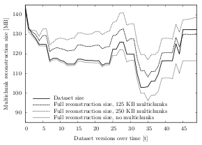 | 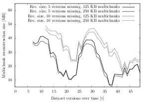 |
| Figure 6.20: Full reconstruction size over time, clustered by multichunk size (dataset C). | Figure 6.21: Reconstruction size over time, clustered by missing versions and multichunk size (dataset C). |
Independent of the multichunk size, the full reconstruction size for dataset C is almost always larger than the actual size of the dataset. Compared to that, reconstructing the dataset version without the use of multichunks always requires downloading fewer data. Figure 6.20 shows that full reconstruction with 125 KB multichunks requires downloading an average of 124 MB for the dataset version, whereas reconstruction with 250 KB multichunks requires on average of 130 MB (difference of only 5%). When reconstructing the version by downloading the individual chunks, the average download volume is 115 MB, which is less than the average size of the dataset version (119 MB).
After an initial full download of a dataset, updating to the latest version requires downloading fewer multichunks. Figure 6.21 shows how many multichunks need to be downloaded to bring the existing version to the latest state. In particular, it shows that the download size grows when more versions are missing in between the local version and the newest version. For dataset C, the average reconstruction size if five versions are missing is 23.7 MB when 125 KB multichunks are used, compared to 22.2 MB when 250 KB multichunks are used. If ten versions are missing, the average reconstruction size for 125 KB multichunks is 34.5 MB and for 250 KB multichunks it is 32.4 MB.
6.6.3.2. Changes over Time
With regard to the multichunk concept, the factor time is of particular importance. Especially when looking at how files are added, changed and removed from a dataset, the differences in the reconstruction behavior are huge. The previous section briefly showed that the reconstruction size depends on the multichunk size. In addition to the multichunk size, the amount and type of changes over time is also relevant.
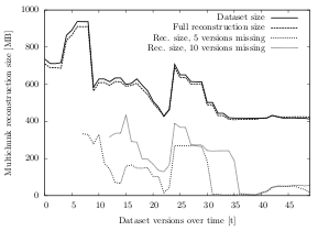 | 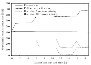 |
| Figure 6.22: Reconstruction size over time, clustered by the number of missing versions (dataset B). | Figure 6.23: Reconstruction size over time, clustered by the number of missing versions (dataset D). |
Looking at dataset B in figure 6.22, for instance, the reconstruction size is significantly lower if there already is a local version present. Over time, when files are altered in the dataset, some of the remote multichunks become partially irrelevant for the reconstruction, while others do not. These partially irrelevant multichunks have to be downloaded completely in order to get the necessary chunks. The more often a dataset is changed, the higher is the amount of data an unsynchronized client has to download for reconstruction. For dataset B, the average reconstruction size is 115 MB if the last five versions are missing and 179 MB if the last ten are missing. Compared to that, the average full reconstruction size is 557 MB, with an average dataset size of 569 MB. If more versions were in between the local and the current version, the average amount would be even higher.
While the full reconstruction size in dataset B is almost always below the respective size of the dataset version, reconstructing dataset D requires a significant overhead. Figure 6.23 shows the multichunk reconstruction size over time for dataset D. With the exception of the initial run, the full reconstruction size is always much higher than the dataset size. After only one additional version, reconstructing version V1 requires downloading 557 MB (overhead of 137 MB to the dataset size, +32.6%). After 19 other versions, this overhead grows to almost double the size of the dataset: For a 424 MB dataset, the client needs to download 778 MB of multichunks (overhead of 354 MB, +83.4%). On average, the full reconstruction size for dataset D is 647 MB.
While the full reconstruction size behaves differently for dataset B and D, it behaves similar when the last five or ten versions are missing: On average, a client needs to download 111 MB to update its local version if five versions are missing and 174 MB if ten are missing.
6.6.3.3. Download Bandwidth
Even though the multichunk concept implies a higher download volume, the bandwidths measured using the DownloadTests application show that the total download time is still shorter when multichunks are used. In particular, the experiments proof that independent of the storage type, using 250 KB multichunks is the best option with regard to the download time.
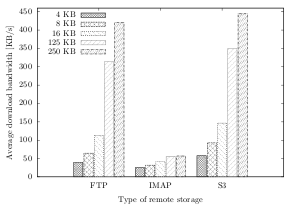 | 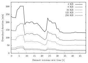 |
| Figure 6.24: Average download bandwidth, clustered by chunk/multichunk size and storage type (all datasets). | Figure 6.25: Average download duration over time, clustered by chunk/multichunk size (dataset B). |
On average, the download speed behaves similar to the upload speed (as measured in experiment 2). Independent of the storage type, the download bandwidth is much higher if multichunks are used (figure 6.24). For FTP (Amazon S3), the average download bandwidth is 39 KB/s (58 KB/s) using 4 KB chunks, compared to 421 KB/s (444 KB/s) using 250 KB multichunks. Similar to the upload speed, the IMAP download bandwidth is much lower than that: Using 4 KB chunks, IMAP only reaches 25 KB/s and only 57 KB/s if 250 KB multichunks are used. The bandwidths of the other chunk/multichunk sizes lie in between those values.
In combination with the reconstruction size per version, the download bandwidths can be used to calculate the total download duration (table 6.9). For the chunk sizes 4 KB, 8 KB and 16 KB, the value of Need-to-Download Chunks was used for the calculation. For the multichunk sizes 125 KB and 250 KB, the value of Need-to-Download Multichunks was used as a basis (cf. equation 6.1).
Table 6.9 shows the results of the estimated download time for each dataset. On average, using 250 KB multichunks is almost three times faster than using 4 KB chunks. When IMAP is excluded from the calculation, the spread in download duration is even higher: Downloading the necessary 4 KB chunks takes about seven times longer than downloading the required 250 KB multichunks.
| Using Chunks | Using Multichunks | ||||||
| 4 KB | 8 KB | 16 KB | 125 KB | 250 KB | |||
| Set A | FTP | 110 sec | 68 sec | 39 sec | 16 sec | 12 sec | |
| IMAP | 172 sec | 138 sec | 109 sec | 89 sec | 86 sec | ||
| Amazon S3 | 75 sec | 48 sec | 30 sec | 14 sec | 11 sec | ||
| Set B | FTP | 224 min | 139 min | 80 min | 29 min | 22 min | |
| IMAP | 350 min | 282 min | 221 min | 168 min | 164 min | ||
| Amazon S3 | 153 min | 97 min | 62 min | 26 min | 21 min | ||
| Set C | FTP | 47 min | 29 min | 17 min | 7 min | 5 min | |
| IMAP | 74 min | 60 min | 48 min | 38 min | 38 min | ||
| Amazon S3 | 32 min | 21 min | 13 min | 6 min | 5 min | ||
| Set D | FTP | 177 min | 108 min | 62 min | 35 min | 25 min | |
| IMAP | 277 min | 219 min | 171 min | 201 min | 187 min | ||
| Amazon S3 | 121 min | 76 min | 48 min | 32 min | 24 min | ||
Table 6.9: Calculated average dataset download times, clustered by chunk/multichunk size, dataset and storage type.
Looking at dataset D, for instance, the average download time using FTP and 4 KB chunks is about 176 minutes (almost 3 hours) for 420 MB of chunks. Compared to that, downloading the necessary 250 KB multichunks for reconstruction only takes 25 minutes – even though almost 640 MB multichunks need to be downloaded. Similarly, reconstructing a version in dataset B using Amazon S3 and 4 KB chunks takes about 153 minutes (2.5 hours; 530 MB chunk data), while downloading the 560 MB multichunk data only takes 21 minutes (250 KB multichunks).
Figure 6.25 shows these different download times for dataset B over time for an FTP storage: For each of the versions in dataset B, downloading the necessary chunks/multichunks takes only about 25–50 minutes if 125/250 KB multichunks are used, but always over two hours if the data is stored in 4 KB chunks. On average, downloading the necessary chunk data takes about 3.7 hours if 4 KB chunks are used and about 22 minutes if the repository stores 250 KB chunks.
6.6.4. Discussion
Experiments 1 and 2 have shown that the multichunk concept greatly improves the upload bandwidth and overall upload time. With the use of multichunks, the total amounts of uploaded data as well as the upload latency are minimized.
Contrary to the positive results of the previous two experiments, experiment 3 has shown that the effects on the download size are rather negative. In particular, when multichunks are used, the average reconstruction size is significantly larger than without the use of multichunks.
In the extreme case of dataset D, for instance, the amount a client needs to download to update its local version of the dataset is sometimes double the size of the actual dataset. In addition to that, this effect gets worse over time and can grow by the order of magnitudes.
Consider the following example: A user creates 250 1 KB files and synchronizes these files to a Syncany repository using 250 KB multichunks. In this case, Syncany creates one 250 KB multichunk containing all of the 250 files. In the next run, the user removes 249 of these 1 KB files and adds 250 new 1 KB files. Syncany knows one of the files and adds the 250 new files to a new multichunk. The user then removes 249 of the 250 newly added files and repeats this action 250 times. In this case, the 250 1 KB files of the last run are distributed over 250 multichunks. If a user wants to reconstruct this dataset version, he or she needs to download all of these multichunks to extract the 1 KB that is needed form each of them. That is a total of 250 times 250 KB needs to be downloaded (62.5 MB). Scaled up to more than one multichunk in the initial run, the overall concept quickly gets unfeasible for everyday use.
However, while the worst case scenario shows an extremely bad behavior, the experiments show very good results in terms of download duration: Even with the significant download overhead due to the multichunks, the download time is still lower if multichunks are used. In fact, the higher average download speed for 125/250 KB multichunks counteracts the additional overhead in almost all cases.
From a user’s perspective, the download time is in most cases more important than the amount of downloaded data. For Syncany users, a minimal download time means a shortened synchronization time between different Syncany clients. Especially when many users are working on the same files, both upload and download time should be minimal. However, in some cases, traffic is paid by the user and can hence be more important than synchronization time. If Amazon S3 is used as remote storage, for instance, download traffic costs around 1ct/GB, whereas the per-request cost is only a fraction of that.
In addition to the traffic overhead caused by larger multichunks, the concept can produce a higher storage volume as well. Especially over time, when some of the multichunks become partially irrelevant for the reconstruction of the last n versions, they cannot be deleted until none of the chunks in the multichunk are needed anymore. Looking at dataset D (Linux kernel sources), for instance, the cause of this effect becomes more obvious. Contrary to other datasets, source code repositories often include some small files that almost never change (e.g. license or readme files). In the initial run, these files are chunked and bundled in multichunks with many other files. Over time, while all the other files in the multichunk get updated or deleted, these few files do not change and continue to be stored in their multichunk – thereby causing additional download overhead (traffic costs) and requiring more storage space. Without additional cleanup methods (e.g. re-grouping chunks from multichunks with a high percentage of superfluous chunks to new multichunks), the costs can quickly become higher than expected.
However, with one of the goals being a minimal synchronization time, the overall results are largely positive: As described above, the overhead caused by larger multichunks was expected to negatively influence the download time. Larger chunks and multichunks were expected to imply a longer download time. Instead the effects are quite the opposite. The reduction of requests also reduces the latency and thereby minimizes the download time. For Syncany users, that means that 250 KB multichunks are not only the best option in terms of chunking efficiency and upload time, but also in terms of reconstruction time.
» Next chapter: Future Research
* 1 Due to the pre-alpha state of Syncany and the complexity of running the data analysis tool (cf. [appendix B](/blog/minimizing-remote-storage-usage-and-synchronization-time-using-deduplication-and-multichunking-syncany-as-an-example/)), the results indicate a fairly large number of technical users -- particularly developers.
* 2 Due to the large amount of possible file types, the pre-study analysis tool only considered the extensions of a file (e.g. .jpg) and not its actual file signature.
* 3 This includes the file extensions doc, docx, xls, xlsx, ppt, pptx, odt, ods, odp and rtf.
* 4 Multichunk compression occurs after the chunking process and has therefore no influence on the chunking duration. Instead, the total duration is used for comparison. See [appendix C](/blog/minimizing-remote-storage-usage-and-synchronization-time-using-deduplication-and-multichunking-syncany-as-an-example/) for a detailed explanation.
* 5 As with the compression parameter, the write pause parameter is independent of the chunking process: The duration in the graph is the total duration and _not_ the chunking duration.
* <a id="Footnote-6"></a> 6 The _write pause_ parameter is not relevant for the analysis of the deduplication ratio, because the ratio is identical for both values (0 ms and 30 ms). Hence, the number of configurations in this regard is 72 and not 144.
* <a id="Footnote-7"></a> 7 This discussion assumes a user workstation such as a desktop or a laptop. If Syncany is used as daemon on a server machine, prerequisites might be different.
* <a id="Footnote-8"></a> 8 Due to a miscalculation in experiment 1, the experiment had to be repeated for the reconstruction data. Instead of running all 72 configurations for the calculation of experiment 3, only twelve were used. The algorithms were selected from the deduplication ranking (equally distributed).
Download as PDF: This article is a web version of my Master’s thesis. Feel free to download the original PDF version.
7. Future Research
Looking at all of the experiments, the overall goal of the thesis has been more than fulfilled: The selected algorithm performs well in terms of chunking efficiency and also improves the synchronization time of Syncany clients. However, given the complexity of the system and its proximity to other research areas, there are many possibilities for future research.
A necessity to make Syncany ready for end-user machines is to make its CPU usage acceptable. While this thesis tried reducing processor usage, it failed to introduce a hard limit for maximum CPU usage. As mentioned in previous chapters, one possibility to solve this problem is to use a dynamic write pause parameter instead of a static one. However, other options might also be possible and can be further researched.
In terms of resource usage, this thesis only analyzed the processor performance and not the use of disk I/O or memory. Especially RAM usage, however, is crucial when an in-memory index is used. Future research might hence focus on optimizing memory usage, for example with the help of techniques such as extreme binning [14].
Given the amount of possible input parameters identified by the thesis, the experiments were not able to test all of the possible combinations. For a complete analysis, however, the other parameter values must be included in the experiments. In fact, there might be other parameters that this thesis did not take into account. Research could focus on further improving the chunking efficiency with a more complete set of parameters. Instead of testing each of the algorithms, a future analysis could use evolutionary methods to find the best combination.
Besides theoretical research, Syncany needs to be tested with real user data on real user machines. Possible future work could include tests of Syncany in real-life scenarios.
Download as PDF: This article is a web version of my Master’s thesis. Feel free to download the original PDF version.
8. Conclusion
File synchronization applications such as Dropbox and Jungle Disk have become increasingly popular in the last few years. While they allow easy file sharing among participating users, they strongly depend on a provider and lack confidentiality.
This thesis introduced Syncany, a file synchronizer designed with security and provider independence as a core part of its architecture. Syncany provides the same functionality as other file synchronizers, but encrypts files locally before uploading and supports any kind of storage. The core processes in Syncany are based on deduplication, a technology that drastically reduces the amount of storage required on the remote servers and at the same time enables versioning capabilities.
The key goal of this thesis was to determine the suitability of deduplication for end-user applications. In particular, the goals for the example of Syncany were to find a suitable deduplication algorithm for the application and to minimize synchronization time among Syncany clients.
To determine the best algorithm for Syncany, the thesis performed experiments on four different datasets. Experiment 1 focused on reducing the amount of required storage on the remote servers. By varying six different algorithm parameters, it analyzed 144 algorithm configurations in terms of deduplication ratio, CPU usage and duration. The experiment found that some of the parameters have a high influence on these measures and others hardly make a difference.
The most important factor when performing deduplication on a client is the fact that calculations are very CPU intensive: While the experiments have not found any algorithms with an acceptable level of CPU usage, they have identified the write pause parameter as the key factor to reduce processor usage. More specifically, none of the tested write pause values were able to lower the CPU usage to the desired level, but the concept of the parameter has proven to be effective and allows the possibility of future research.
In terms of deduplication ratio, the fingerprinting algorithm Adler-32 has a high impact on the efficiency of the deduplication algorithm. In combination with the variable-size chunking method TTTD, Adler-32 has achieved remarkable space savings in the experiments and outperforms other fingerprinters by the order of magnitude. To the best of the author’s knowledge, Adler-32 has not been used as a fingerprinter in other deduplication systems so far.
Experiments 2 and 3 focused on reducing the overall synchronization time between Syncany clients. By transferring chunks and multichunks resulting from the deduplication algorithms to the remote storage, the experiments measured the time and bandwidth implied by each algorithm configuration. The results show that independent of the storage type, the multichunk concept is invaluable to the Syncany architecture. By combining chunks to multichunks, both upload and download time have shown to be decreased significantly on all of the analyzed types of remote storage. While the results indicate a higher reconstruction size when the size of the multichunks is increased, downloading large multichunks is still faster than downloading small chunks with high per-request latency.
In conclusion, all of the experiments show that deduplication is a valid technology for end-user applications if controlled properly and combined with other concepts. Especially in the case of Syncany, in which the storage abstraction prohibits the use of server-side software, deduplication cannot function properly without additional data processing. As demonstrated in the experiments, the multichunk concept fulfills this role by adding chunks to a container format before uploading. Using multichunks, the deduplication ratio can be further increased and the synchronization time has shown to be reduced significantly. The experiments have also demonstrated that without the use of multichunks, the upload and download time for Syncany clients would be unfeasible to end-users.
With regard to the overall goal of the thesis, the selected algorithm has shown to be very effective on all of the datasets. It offers a good trade-off between chunking efficiency, processor usage and duration. At the same time, it reduces the total synchronization time between Syncany clients.
» Next chapter: Appendix “List of Configurations”
Download as PDF: This article is a web version of my Master’s thesis. Feel free to download the original PDF version.
A. List of Configurations
The following list represents the chunking/multichunking configurations which have been compared in the experiments in chapter 5.
| Custom-125-0/Fixed-4/Cipher Custom-125-0/TTTD-4-Adler32/Cipher Custom-125-0/TTTD-4-PLAIN/Cipher Custom-125-0/TTTD-4-Rabin/Cipher Custom-125-0/Fixed-8/Cipher Custom-125-0/TTTD-8-Adler32/Cipher Custom-125-0/TTTD-8-PLAIN/Cipher Custom-125-0/TTTD-8-Rabin/Cipher Custom-125-0/Fixed-16/Cipher Custom-125-0/TTTD-16-Adler32/Cipher Custom-125-0/TTTD-16-PLAIN/Cipher Custom-125-0/TTTD-16-Rabin/Cipher Custom-125-0/Fixed-4/Gzip-Cipher Custom-125-0/TTTD-4-Adler32/Gzip-Cipher Custom-125-0/TTTD-4-PLAIN/Gzip-Cipher Custom-125-0/TTTD-4-Rabin/Gzip-Cipher Custom-125-0/Fixed-8/Gzip-Cipher Custom-125-0/TTTD-8-Adler32/Gzip-Cipher Custom-125-0/TTTD-8-PLAIN/Gzip-Cipher Custom-125-0/TTTD-8-Rabin/Gzip-Cipher Custom-125-0/Fixed-16/Gzip-Cipher Custom-125-0/TTTD-16-Adler32/Gzip-Cipher Custom-125-0/TTTD-16-PLAIN/Gzip-Cipher Custom-125-0/TTTD-16-Rabin/Gzip-Cipher Custom-125-0/Fixed-4/Bzip2-Cipher Custom-125-0/TTTD-4-Adler32/Bzip2-Cipher Custom-125-0/TTTD-4-PLAIN/Bzip2-Cipher Custom-125-0/TTTD-4-Rabin/Bzip2-Cipher Custom-125-0/Fixed-8/Bzip2-Cipher Custom-125-0/TTTD-8-Adler32/Bzip2-Cipher Custom-125-0/TTTD-8-PLAIN/Bzip2-Cipher Custom-125-0/TTTD-8-Rabin/Bzip2-Cipher Custom-125-0/Fixed-16/Bzip2-Cipher Custom-125-0/TTTD-16-Adler32/Bzip2-Cipher Custom-125-0/TTTD-16-PLAIN/Bzip2-Cipher Custom-125-0/TTTD-16-Rabin/Bzip2-Cipher Custom-250-0/Fixed-4/Cipher Custom-250-0/TTTD-4-Adler32/Cipher Custom-250-0/TTTD-4-PLAIN/Cipher Custom-250-0/TTTD-4-Rabin/Cipher Custom-250-0/Fixed-8/Cipher Custom-250-0/TTTD-8-Adler32/Cipher Custom-250-0/TTTD-8-PLAIN/Cipher Custom-250-0/TTTD-8-Rabin/Cipher Custom-250-0/Fixed-16/Cipher Custom-250-0/TTTD-16-Adler32/Cipher Custom-250-0/TTTD-16-PLAIN/Cipher Custom-250-0/TTTD-16-Rabin/Cipher Custom-250-0/Fixed-4/Gzip-Cipher Custom-250-0/TTTD-4-Adler32/Gzip-Cipher Custom-250-0/TTTD-4-PLAIN/Gzip-Cipher Custom-250-0/TTTD-4-Rabin/Gzip-Cipher Custom-250-0/Fixed-8/Gzip-Cipher Custom-250-0/TTTD-8-Adler32/Gzip-Cipher Custom-250-0/TTTD-8-PLAIN/Gzip-Cipher Custom-250-0/TTTD-8-Rabin/Gzip-Cipher Custom-250-0/Fixed-16/Gzip-Cipher Custom-250-0/TTTD-16-Adler32/Gzip-Cipher Custom-250-0/TTTD-16-PLAIN/Gzip-Cipher Custom-250-0/TTTD-16-Rabin/Gzip-Cipher Custom-250-0/Fixed-4/Bzip2-Cipher Custom-250-0/TTTD-4-Adler32/Bzip2-Cipher Custom-250-0/TTTD-4-PLAIN/Bzip2-Cipher Custom-250-0/TTTD-4-Rabin/Bzip2-Cipher Custom-250-0/Fixed-8/Bzip2-Cipher Custom-250-0/TTTD-8-Adler32/Bzip2-Cipher Custom-250-0/TTTD-8-PLAIN/Bzip2-Cipher Custom-250-0/TTTD-8-Rabin/Bzip2-Cipher Custom-250-0/Fixed-16/Bzip2-Cipher Custom-250-0/TTTD-16-Adler32/Bzip2-Cipher Custom-250-0/TTTD-16-PLAIN/Bzip2-Cipher Custom-250-0/TTTD-16-Rabin/Bzip2-Cipher Custom-125-20/Fixed-4/Cipher Custom-125-20/TTTD-4-Adler32/Cipher Custom-125-20/TTTD-4-PLAIN/Cipher Custom-125-20/TTTD-4-Rabin/Cipher | Custom-125-20/Fixed-8/Cipher Custom-125-20/TTTD-8-Adler32/Cipher Custom-125-20/TTTD-8-PLAIN/Cipher Custom-125-20/TTTD-8-Rabin/Cipher Custom-125-20/Fixed-16/Cipher Custom-125-20/TTTD-16-Adler32/Cipher Custom-125-20/TTTD-16-PLAIN/Cipher Custom-125-20/TTTD-16-Rabin/Cipher Custom-125-20/Fixed-4/Gzip-Cipher Custom-125-20/TTTD-4-Adler32/Gzip-Cipher Custom-125-20/TTTD-4-PLAIN/Gzip-Cipher Custom-125-20/TTTD-4-Rabin/Gzip-Cipher Custom-125-20/Fixed-8/Gzip-Cipher Custom-125-20/TTTD-8-Adler32/Gzip-Cipher Custom-125-20/TTTD-8-PLAIN/Gzip-Cipher Custom-125-20/TTTD-8-Rabin/Gzip-Cipher Custom-125-20/Fixed-16/Gzip-Cipher Custom-125-20/TTTD-16-Adler32/Gzip-Cipher Custom-125-20/TTTD-16-PLAIN/Gzip-Cipher Custom-125-20/TTTD-16-Rabin/Gzip-Cipher Custom-125-20/Fixed-4/Bzip2-Cipher Custom-125-20/TTTD-4-Adler32/Bzip2-Cipher Custom-125-20/TTTD-4-PLAIN/Bzip2-Cipher Custom-125-20/TTTD-4-Rabin/Bzip2-Cipher Custom-125-20/Fixed-8/Bzip2-Cipher Custom-125-20/TTTD-8-Adler32/Bzip2-Cipher Custom-125-20/TTTD-8-PLAIN/Bzip2-Cipher Custom-125-20/TTTD-8-Rabin/Bzip2-Cipher Custom-125-20/Fixed-16/Bzip2-Cipher Custom-125-20/TTTD-16-Adler32/Bzip2-Cipher Custom-125-20/TTTD-16-PLAIN/Bzip2-Cipher Custom-125-20/TTTD-16-Rabin/Bzip2-Cipher Custom-250-20/Fixed-4/Cipher Custom-250-20/TTTD-4-Adler32/Cipher Custom-250-20/TTTD-4-PLAIN/Cipher Custom-250-20/TTTD-4-Rabin/Cipher Custom-250-20/Fixed-8/Cipher Custom-250-20/TTTD-8-Adler32/Cipher Custom-250-20/TTTD-8-PLAIN/Cipher Custom-250-20/TTTD-8-Rabin/Cipher Custom-250-20/Fixed-16/Cipher Custom-250-20/TTTD-16-Adler32/Cipher Custom-250-20/TTTD-16-PLAIN/Cipher Custom-250-20/TTTD-16-Rabin/Cipher Custom-250-20/Fixed-4/Gzip-Cipher Custom-250-20/TTTD-4-Adler32/Gzip-Cipher Custom-250-20/TTTD-4-PLAIN/Gzip-Cipher Custom-250-20/TTTD-4-Rabin/Gzip-Cipher Custom-250-20/Fixed-8/Gzip-Cipher Custom-250-20/TTTD-8-Adler32/Gzip-Cipher Custom-250-20/TTTD-8-PLAIN/Gzip-Cipher Custom-250-20/TTTD-8-Rabin/Gzip-Cipher Custom-250-20/Fixed-16/Gzip-Cipher Custom-250-20/TTTD-16-Adler32/Gzip-Cipher Custom-250-20/TTTD-16-PLAIN/Gzip-Cipher Custom-250-20/TTTD-16-Rabin/Gzip-Cipher Custom-250-20/Fixed-4/Bzip2-Cipher Custom-250-20/TTTD-4-Adler32/Bzip2-Cipher Custom-250-20/TTTD-4-PLAIN/Bzip2-Cipher Custom-250-20/TTTD-4-Rabin/Bzip2-Cipher Custom-250-20/Fixed-8/Bzip2-Cipher Custom-250-20/TTTD-8-Adler32/Bzip2-Cipher Custom-250-20/TTTD-8-PLAIN/Bzip2-Cipher Custom-250-20/TTTD-8-Rabin/Bzip2-Cipher Custom-250-20/Fixed-16/Bzip2-Cipher Custom-250-20/TTTD-16-Adler32/Bzip2-Cipher Custom-250-20/TTTD-16-PLAIN/Bzip2-Cipher Custom-250-20/TTTD-16-Rabin/Bzip2-Cipher |
» Next chapter: Appendix “Pre-Study Folder Statistics”
Download as PDF: This article is a web version of my Master’s thesis. Feel free to download the original PDF version.
B. Pre-Study Folder Statistics
To get a better idea of what kind of data users will be storing inside the Syncany folders, the pre-study asked users and developers to run a small java program to collect data about the files types and sizes. In particular, they were asked to run the following commands on a folder that contains the type of files they would store in Syncany. Because many of them might use Dropbox, they were given the option to choose the Dropbox folder.
wget http://syncany.org/thesis/FileTreeStatCSV.java
javac FileTreeStatCSV.java
java FileTreeStatCSV ~/SomeFolder
Analyzing directory /home/username/SomeFolder ...
Saving to syncany-size-categories.csv ...
Saving to syncany-type-categories.csv ...
After running the commands, they were asked to upload the CSV files using the an interface on the Syncany Web site. The program generated two CSV files – one containing data about the file types, and one representing a histogram of existing file sizes:
Excerpt of syncany-type-categories.csv:fileExt,totalFileCount,totalFileSize
bmp,1,1025442
jpg,9,7772374
pdf,3,244802
doc,110,2044928
docx,1,35428
... | Excerpt of syncany-size-categories.csv:fileSizeCategory,totalFileCount
128,36
256,14
512,38
1000,46
2000,38
... |
» Next chapter: Appendix “List of Variables Recorded”
Download as PDF: This article is a web version of my Master’s thesis. Feel free to download the original PDF version.
C. List of Variables Recorded
The following table contains a detailed explanation of each variable recorded in experiment 1 (cf. chapter 6.4.1). For each dataset version and each configuration, one set of these variables was saved.
| Measured Variable | Description |
| totalDurationSec | Duration of the chunking and indexing process for the run |
| totalChunkingDurationSec | Duration of the chunking process for the run (excludes index lookups and other management tasks) |
| totalDatasetFileCount | Number of analyzed files in the run, i.e. the number of files in this version of the dataset |
| totalChunkCount | Number of created chunks from the files analyzed |
| totalDatasetSize | Size in bytes of all analyzed files in the run |
| totalNewChunkCount | Number of chunks that have not been found in the index (new chunks, negative chunk index lookup) |
| totalNewChunkSize | Size in bytes of all the new chunks |
| totalNewFileCount | Number of new files (negative file index lookup) |
| totalNewFileSize | Size in bytes of all the new files |
| totalDuplicateChunkCount | Number of chunks that have been found in the index (positive chunk index lookup) |
| totalDuplicateChunkSize | Size in bytes of all duplicate chunks |
| totalDuplicateFileCount | Number of duplicate files found during this run (positive file index lookup) |
| totalDuplicateFileSize | Size in bytes of duplicate files during this run |
| totalMultiChunkCount | Number of multichunks created from the new chunks |
| totalMultiChunkSize | Size in bytes of the created multichunks |
| totalIndexSize | Size in bytes of the incremental index file for this run |
| totalCpuUsage | CPU usage during this run in percent |
| tempDedupRatio | Temporal deduplication ratio, excluding the size of the index; calculated by dividing the sum of the cumulated input bytes by the cumulated size of the generated multichunks in bytes (both from t0 to tn) |
| tempSpaceReducationRatio | Temporal space reduction in percent, excluding the size of the index; calculated as one minus the inverse temporal deduplication ratio |
| tempDedupRatioInclIndex | Temporal deduplication ratio, incl. the size of the index |
| tempSpaceRedRatioInclIndex | Temporal space reduction in percent, including the size of the index |
| recnstChunksNeedBytes | Size in bytes of chunks needed to reconstruct the current dataset version if no previous version has been downloaded before |
| recnstMultChnksNeedBytes | Size in bytes of multichunks needed to reconstruct the current dataset version if no previous version has been downloaded before |
| recnstMultOverhDiffBytes | Difference in bytes between required size of multichunks and size of chunks. |
| recnst5NeedMultChnkBytes | Size in bytes of multichunks needed to reconstruct the current dataset version if the last five dataset versions are missing |
| recnst5NeedChunksBytes | Size in bytes of chunks needed to reconstruct the current dataset version if the last five dataset versions are missing |
| recnst5OverheadBytes | Difference in bytes between required size of multichunks and size of chunks (if five versions are missing). |
| recnst10NeedMultChnkBytes | Size in bytes of multichunks needed to reconstruct the current dataset version if the last ten dataset versions are missing |
| recnst10NeedChunksBytes | Size in bytes of chunks needed to reconstruct the current dataset version if the last ten dataset versions are missing |
| recnst10OverhBytes | Difference in bytes between required size of multichunks and size of chunks (if ten versions are missing). |
Table C.1: Variables recorded for each dataset version during experiment 1.
» Next chapter: Appendix “Best Algorithms by Deduplication Ratio”
Download as PDF: This article is a web version of my Master’s thesis. Feel free to download the original PDF version.
D. Best Algorithms by Deduplication Ratio
The following table lists the best algorithm configurations with regard to the deduplication ratio. The list is sorted by the average temporal deduplication ratio (last column). All values are deduplication ratios (ratio:1).
| Rank | Algorithm Configuration | A | B | C | D | Average | |
| 1 | Custom-250-*/TTTD-4-Adler32/Bzip2-Cipher | 15.35 | 12.88 | 15.43 | 32.67 | 16.68 | |
| 2 | Custom-125-*/TTTD-4-Adler32/Bzip2-Cipher | 15.33 | 12.84 | 15.40 | 30.92 | 16.45 | |
| 3 | Custom-250-*/TTTD-8-Adler32/Bzip2-Cipher | 15.13 | 12.80 | 15.00 | 30.56 | 16.22 | |
| 4 | Custom-250-*/TTTD-4-Adler32/Gzip-Cipher | 15.37 | 12.82 | 15.37 | 28.31 | 16.14 | |
| 5 | Custom-125-*/TTTD-4-Adler32/Gzip-Cipher | 15.39 | 12.82 | 15.38 | 27.99 | 16.11 | |
| 6 | Custom-125-*/TTTD-8-Adler32/Bzip2-Cipher | 15.12 | 12.75 | 14.96 | 29.00 | 16.01 | |
| 7 | Custom-250-*/TTTD-16-Adler32/Bzip2-Cipher | 14.55 | 12.67 | 14.68 | 28.74 | 15.71 | |
| 8 | Custom-250-*/TTTD-8-Adler32/Gzip-Cipher | 15.16 | 12.73 | 14.94 | 26.37 | 15.70 | |
| 9 | Custom-125-*/TTTD-8-Adler32/Gzip-Cipher | 15.17 | 12.73 | 14.94 | 26.11 | 15.67 | |
| 10 | Custom-125-*/TTTD-16-Adler32/Bzip2-Cipher | 14.53 | 12.63 | 14.66 | 27.29 | 15.51 | |
| 11 | Custom-250-*/TTTD-16-Adler32/Gzip-Cipher | 14.57 | 12.59 | 14.61 | 24.68 | 15.19 | |
| 12 | Custom-125-*/TTTD-16-Adler32/Gzip-Cipher | 14.58 | 12.59 | 14.63 | 24.44 | 15.17 | |
| 13 | Custom-250-*/TTTD-4-PLAIN/Bzip2-Cipher | 6.73 | 12.21 | 12.72 | 34.19 | 13.33 | |
| 14 | Custom-125-*/TTTD-4-PLAIN/Bzip2-Cipher | 6.72 | 12.15 | 12.68 | 32.33 | 13.08 | |
| 15 | Custom-250-*/TTTD-8-PLAIN/Bzip2-Cipher | 6.79 | 12.14 | 11.75 | 32.91 | 12.90 | |
| 16 | Custom-250-*/TTTD-4-Adler32/Cipher | 15.12 | 12.07 | 13.54 | 7.00 | 12.80 | |
| 17 | Custom-125-*/TTTD-4-Adler32/Cipher | 15.12 | 12.07 | 13.54 | 7.00 | 12.80 | |
| 18 | Custom-250-*/TTTD-4-PLAIN/Gzip-Cipher | 6.74 | 12.12 | 12.68 | 29.71 | 12.77 | |
| 19 | Custom-125-*/TTTD-4-PLAIN/Gzip-Cipher | 6.74 | 12.12 | 12.67 | 29.37 | 12.73 | |
| 20 | Custom-125-*/TTTD-8-PLAIN/Bzip2-Cipher | 6.78 | 12.09 | 11.71 | 31.09 | 12.65 | |
| 21 | Custom-250-*/TTTD-8-Adler32/Cipher | 14.90 | 11.95 | 13.08 | 6.45 | 12.50 | |
| 22 | Custom-125-*/TTTD-8-Adler32/Cipher | 14.90 | 11.95 | 13.07 | 6.45 | 12.50 | |
| 23 | Custom-250-*/TTTD-8-PLAIN/Gzip-Cipher | 6.80 | 12.06 | 11.61 | 28.50 | 12.32 | |
| 24 | Custom-125-*/TTTD-8-PLAIN/Gzip-Cipher | 6.80 | 12.05 | 11.61 | 28.13 | 12.27 | |
| 25 | Custom-250-*/Fixed-4/Bzip2-Cipher | 6.64 | 12.13 | 11.39 | 27.90 | 12.15 | |
| 26 | Custom-250-*/Fixed-8/Bzip2-Cipher | 6.61 | 12.16 | 11.41 | 27.76 | 12.14 | |
| 27 | Custom-250-*/TTTD-16-Adler32/Cipher | 14.33 | 11.80 | 12.74 | 5.98 | 12.14 | |
| 28 | Custom-125-*/TTTD-16-Adler32/Cipher | 14.33 | 11.80 | 12.74 | 5.98 | 12.14 | |
| 29 | Custom-250-*/Fixed-16/Bzip2-Cipher | 6.54 | 12.16 | 11.41 | 27.17 | 12.05 | |
| 30 | Custom-125-*/Fixed-4/Bzip2-Cipher | 6.63 | 12.08 | 11.35 | 26.39 | 11.94 | |
| 31 | Custom-125-*/Fixed-8/Bzip2-Cipher | 6.60 | 12.10 | 11.37 | 26.23 | 11.93 | |
| 32 | Custom-250-*/TTTD-16-PLAIN/Bzip2-Cipher | 6.39 | 12.16 | 11.37 | 26.26 | 11.89 | |
| 33 | Custom-125-*/Fixed-16/Bzip2-Cipher | 6.53 | 12.11 | 11.37 | 25.76 | 11.86 | |
| 34 | Custom-250-*/TTTD-8-Rabin/Bzip2-Cipher | 5.32 | 12.10 | 11.73 | 27.28 | 11.78 | |
| 35 | Custom-250-*/TTTD-16-Rabin/Bzip2-Cipher | 6.09 | 12.10 | 11.11 | 26.82 | 11.77 | |
| 36 | Custom-125-*/TTTD-16-PLAIN/Bzip2-Cipher | 6.38 | 12.10 | 11.34 | 24.98 | 11.71 | |
| 37 | Custom-250-*/Fixed-4/Gzip-Cipher | 6.65 | 12.05 | 11.26 | 24.13 | 11.65 | |
| 38 | Custom-250-*/Fixed-8/Gzip-Cipher | 6.62 | 12.07 | 11.28 | 23.90 | 11.63 | |
| 39 | Custom-125-*/Fixed-4/Gzip-Cipher | 6.65 | 12.05 | 11.25 | 23.85 | 11.62 | |
| 40 | Custom-125-*/TTTD-16-Rabin/Bzip2-Cipher | 6.07 | 12.05 | 11.08 | 25.51 | 11.59 | |
| 41 | Custom-125-*/Fixed-8/Gzip-Cipher | 6.62 | 12.07 | 11.27 | 23.60 | 11.59 | |
| 42 | Custom-125-*/TTTD-8-Rabin/Bzip2-Cipher | 5.30 | 12.05 | 11.69 | 25.87 | 11.59 | |
| 43 | Custom-250-*/Fixed-16/Gzip-Cipher | 6.55 | 12.08 | 11.27 | 23.32 | 11.54 | |
| 44 | Custom-125-*/Fixed-16/Gzip-Cipher | 6.56 | 12.07 | 11.27 | 23.08 | 11.51 | |
| 45 | Custom-250-*/TTTD-16-PLAIN/Gzip-Cipher | 6.40 | 12.07 | 11.23 | 22.43 | 11.37 | |
| 46 | Custom-250-*/TTTD-4-Rabin/Bzip2-Cipher | 4.02 | 12.12 | 11.47 | 27.50 | 11.36 | |
| 47 | Custom-125-*/TTTD-16-PLAIN/Gzip-Cipher | 6.41 | 12.06 | 11.23 | 22.23 | 11.35 | |
| 48 | Custom-250-*/TTTD-8-Rabin/Gzip-Cipher | 5.33 | 12.01 | 11.56 | 23.48 | 11.26 | |
| 49 | Custom-250-*/TTTD-16-Rabin/Gzip-Cipher | 6.09 | 12.01 | 10.94 | 22.99 | 11.25 | |
| 50 | Custom-125-*/TTTD-8-Rabin/Gzip-Cipher | 5.32 | 12.01 | 11.55 | 23.23 | 11.23 | |
| 51 | Custom-125-*/TTTD-16-Rabin/Gzip-Cipher | 6.10 | 12.01 | 10.93 | 22.79 | 11.22 | |
| 52 | Custom-125-*/TTTD-4-Rabin/Bzip2-Cipher | 4.01 | 12.07 | 11.43 | 26.02 | 11.15 | |
| 53 | Custom-250-*/TTTD-4-Rabin/Gzip-Cipher | 4.03 | 12.04 | 11.34 | 23.77 | 10.85 | |
| 54 | Custom-125-*/TTTD-4-Rabin/Gzip-Cipher | 4.03 | 12.03 | 11.33 | 23.49 | 10.82 | |
| 55 | Custom-250-*/TTTD-4-PLAIN/Cipher | 6.66 | 11.44 | 11.30 | 7.37 | 9.51 | |
| 56 | Custom-125-*/TTTD-4-PLAIN/Cipher | 6.66 | 11.44 | 11.30 | 7.37 | 9.51 | |
| 57 | Custom-250-*/TTTD-8-PLAIN/Cipher | 6.71 | 11.31 | 10.10 | 6.99 | 9.09 | |
| 58 | Custom-125-*/TTTD-8-PLAIN/Cipher | 6.71 | 11.31 | 10.10 | 6.99 | 9.09 | |
| 59 | Custom-250-*/Fixed-4/Cipher | 6.58 | 11.33 | 9.82 | 5.92 | 8.85 | |
| 60 | Custom-125-*/Fixed-4/Cipher | 6.58 | 11.33 | 9.82 | 5.91 | 8.85 | |
| 61 | Custom-250-*/Fixed-8/Cipher | 6.54 | 11.34 | 9.80 | 5.79 | 8.82 | |
| 62 | Custom-125-*/Fixed-8/Cipher | 6.54 | 11.34 | 9.80 | 5.79 | 8.82 | |
| 63 | Custom-250-*/Fixed-16/Cipher | 6.47 | 11.32 | 9.78 | 5.62 | 8.77 | |
| 64 | Custom-125-*/Fixed-16/Cipher | 6.47 | 11.32 | 9.78 | 5.62 | 8.77 | |
| 65 | Custom-250-*/TTTD-16-PLAIN/Cipher | 6.31 | 11.28 | 9.71 | 5.37 | 8.66 | |
| 66 | Custom-125-*/TTTD-16-PLAIN/Cipher | 6.31 | 11.28 | 9.71 | 5.37 | 8.66 | |
| 67 | Custom-250-*/TTTD-16-Rabin/Cipher | 6.00 | 11.23 | 9.31 | 5.53 | 8.46 | |
| 68 | Custom-125-*/TTTD-16-Rabin/Cipher | 6.00 | 11.23 | 9.31 | 5.53 | 8.46 | |
| 69 | Custom-250-*/TTTD-8-Rabin/Cipher | 5.26 | 11.24 | 9.81 | 5.67 | 8.40 | |
| 70 | Custom-125-*/TTTD-8-Rabin/Cipher | 5.26 | 11.24 | 9.81 | 5.67 | 8.40 | |
| 71 | Custom-250-*/TTTD-4-Rabin/Cipher | 3.99 | 11.27 | 9.74 | 5.79 | 8.03 | |
| 72 | Custom-125-*/TTTD-4-Rabin/Cipher | 3.98 | 11.27 | 9.74 | 5.79 | 8.03 |
Table D.1: Average temporal deduplication ratio over all datasets, ordered by the average.
» Next chapter: Appendix “Best Algorithms by Duration”
Download as PDF: This article is a web version of my Master’s thesis. Feel free to download the original PDF version.
E. Best Algorithms by Duration
The following table lists the best algorithm configurations with regard to the overall duration. The list is sorted by the average duration (last column). All values are in seconds.
| Rank | Algorithm Configuration | A | B | C | D | Average |
| 1 | Custom-250-0/Fixed-8/Cipher | 0.10 | 9.09 | 1.70 | 12.92 | 4.72 |
| 2 | Custom-250-0/Fixed-16/Cipher | 0.10 | 8.60 | 1.64 | 14.58 | 4.75 |
| 3 | Custom-125-0/Fixed-16/Cipher | 0.09 | 10.62 | 1.64 | 15.16 | 5.42 |
| 4 | Custom-250-0/Fixed-4/Cipher | 0.10 | 10.88 | 1.88 | 16.82 | 5.76 |
| 5 | Custom-250-0/Fixed-16/Gzip-Cipher | 0.14 | 11.14 | 2.22 | 15.56 | 5.80 |
| 6 | Custom-125-0/Fixed-8/Cipher | 0.10 | 11.99 | 1.71 | 15.13 | 5.84 |
| 7 | Custom-125-0/Fixed-4/Cipher | 0.10 | 10.84 | 1.96 | 17.72 | 5.88 |
| 8 | Custom-125-0/Fixed-16/Gzip-Cipher | 0.14 | 11.00 | 2.20 | 16.91 | 5.91 |
| 9 | Custom-250-0/Fixed-8/Gzip-Cipher | 0.14 | 11.66 | 2.28 | 15.89 | 6.01 |
| 10 | Custom-125-0/Fixed-8/Gzip-Cipher | 0.14 | 11.52 | 2.28 | 17.41 | 6.15 |
| 11 | Custom-125-0/Fixed-4/Gzip-Cipher | 0.15 | 13.33 | 2.43 | 18.46 | 6.85 |
| 12 | Custom-250-0/Fixed-4/Gzip-Cipher | 0.15 | 13.51 | 2.45 | 18.33 | 6.90 |
| 13 | Custom-250-30/Fixed-16/Cipher | 0.19 | 12.53 | 2.63 | 20.29 | 6.90 |
| 14 | Custom-250-30/Fixed-8/Cipher | 0.19 | 12.97 | 2.69 | 20.12 | 7.03 |
| 15 | Custom-250-30/Fixed-4/Cipher | 0.20 | 14.98 | 2.89 | 20.66 | 7.74 |
| 16 | Custom-250-30/Fixed-16/Gzip-Cipher | 0.23 | 14.94 | 3.21 | 22.08 | 8.00 |
| 17 | Custom-250-30/Fixed-8/Gzip-Cipher | 0.24 | 15.62 | 3.27 | 21.37 | 8.14 |
| 18 | Custom-250-0/TTTD-8-PLAIN/Cipher | 0.19 | 17.22 | 4.65 | 20.16 | 8.86 |
| 19 | Custom-125-30/Fixed-16/Cipher | 0.25 | 16.39 | 3.56 | 26.00 | 9.00 |
| 20 | Custom-125-0/TTTD-16-PLAIN/Cipher | 0.19 | 17.24 | 4.69 | 21.28 | 9.01 |
| 21 | Custom-250-0/TTTD-16-PLAIN/Cipher | 0.19 | 17.44 | 4.67 | 21.24 | 9.06 |
| 22 | Custom-125-30/Fixed-8/Cipher | 0.26 | 16.97 | 3.63 | 25.16 | 9.09 |
| 23 | Custom-250-30/Fixed-4/Gzip-Cipher | 0.25 | 17.59 | 3.47 | 24.68 | 9.17 |
| 24 | Custom-250-0/TTTD-4-PLAIN/Cipher | 0.19 | 17.43 | 4.64 | 22.92 | 9.24 |
| 25 | Custom-125-0/TTTD-4-PLAIN/Cipher | 0.19 | 19.50 | 3.49 | 21.81 | 9.38 |
| 26 | Custom-125-0/TTTD-8-PLAIN/Cipher | 0.19 | 19.10 | 4.66 | 20.90 | 9.50 |
| 27 | Custom-125-30/Fixed-4/Cipher | 0.26 | 18.83 | 3.82 | 25.11 | 9.69 |
| 28 | Custom-125-0/TTTD-16-PLAIN/Gzip-Cipher | 0.24 | 19.56 | 5.24 | 23.05 | 10.08 |
| 29 | Custom-250-0/TTTD-8-PLAIN/Gzip-Cipher | 0.23 | 19.68 | 5.21 | 23.31 | 10.13 |
| 30 | Custom-125-0/TTTD-8-PLAIN/Gzip-Cipher | 0.23 | 19.59 | 5.21 | 23.79 | 10.16 |
| 31 | Custom-250-0/TTTD-16-PLAIN/Gzip-Cipher | 0.24 | 19.77 | 5.25 | 24.26 | 10.28 |
| 32 | Custom-125-30/Fixed-8/Gzip-Cipher | 0.31 | 19.75 | 4.26 | 26.87 | 10.31 |
| 33 | Custom-250-0/TTTD-4-PLAIN/Gzip-Cipher | 0.23 | 19.82 | 5.11 | 24.93 | 10.33 |
| 34 | Custom-125-30/Fixed-16/Gzip-Cipher | 0.30 | 19.06 | 4.20 | 29.33 | 10.38 |
| 35 | Custom-125-0/TTTD-4-PLAIN/Gzip-Cipher | 0.23 | 19.82 | 5.10 | 25.41 | 10.39 |
| 36 | Custom-250-0/TTTD-8-Adler32/Cipher | 0.22 | 21.72 | 5.24 | 22.09 | 10.59 |
| 37 | Custom-125-0/TTTD-16-Adler32/Cipher | 0.22 | 21.79 | 5.25 | 22.96 | 10.72 |
| 38 | Custom-250-0/TTTD-16-Adler32/Cipher | 0.22 | 21.79 | 5.21 | 23.28 | 10.74 |
| 39 | Custom-125-0/TTTD-4-Adler32/Cipher | 0.25 | 22.32 | 4.47 | 24.50 | 10.84 |
| 40 | Custom-250-30/TTTD-8-PLAIN/Cipher | 0.27 | 21.19 | 5.59 | 24.62 | 10.85 |
| 41 | Custom-125-0/TTTD-8-Adler32/Cipher | 0.22 | 21.50 | 5.26 | 25.43 | 10.93 |
| 42 | Custom-250-30/TTTD-16-PLAIN/Cipher | 0.28 | 21.04 | 5.63 | 26.40 | 11.03 |
| 43 | Custom-125-30/Fixed-4/Gzip-Cipher | 0.31 | 21.54 | 4.44 | 28.53 | 11.09 |
| 44 | Custom-250-30/TTTD-4-PLAIN/Cipher | 0.28 | 21.48 | 5.45 | 26.91 | 11.17 |
| 45 | Custom-250-0/TTTD-4-Adler32/Cipher | 0.25 | 22.36 | 5.29 | 26.96 | 11.38 |
| 46 | Custom-250-0/TTTD-8-Adler32/Gzip-Cipher | 0.27 | 23.76 | 5.62 | 25.58 | 11.73 |
| 47 | Custom-250-0/TTTD-16-Adler32/Gzip-Cipher | 0.24 | 24.20 | 5.61 | 24.99 | 11.78 |
| 48 | Custom-125-0/TTTD-16-Adler32/Gzip-Cipher | 0.24 | 24.09 | 5.62 | 25.34 | 11.79 |
| 49 | Custom-125-0/TTTD-8-Adler32/Gzip-Cipher | 0.24 | 23.79 | 5.61 | 26.11 | 11.79 |
| 50 | Custom-250-0/TTTD-4-Adler32/Gzip-Cipher | 0.27 | 24.71 | 5.67 | 25.41 | 12.01 |
| 51 | Custom-250-30/TTTD-8-PLAIN/Gzip-Cipher | 0.32 | 23.68 | 6.15 | 27.21 | 12.07 |
| 52 | Custom-125-0/TTTD-4-Adler32/Gzip-Cipher | 0.27 | 24.86 | 5.65 | 26.19 | 12.13 |
| 53 | Custom-250-30/TTTD-16-PLAIN/Gzip-Cipher | 0.33 | 23.55 | 6.23 | 27.93 | 12.14 |
| 54 | Custom-250-30/TTTD-4-PLAIN/Gzip-Cipher | 0.33 | 23.95 | 5.94 | 27.96 | 12.18 |
| 55 | Custom-250-30/TTTD-16-Adler32/Cipher | 0.27 | 25.74 | 5.91 | 27.21 | 12.59 |
| 56 | Custom-250-30/TTTD-8-Adler32/Cipher | 0.30 | 25.45 | 5.92 | 28.31 | 12.65 |
| 57 | Custom-125-30/TTTD-4-PLAIN/Cipher | 0.34 | 25.03 | 6.22 | 30.24 | 12.85 |
| 58 | Custom-250-30/TTTD-4-Adler32/Cipher | 0.30 | 26.15 | 5.97 | 28.50 | 12.89 |
| 59 | Custom-125-30/TTTD-8-PLAIN/Cipher | 0.33 | 24.91 | 6.48 | 31.69 | 13.06 |
| 60 | Custom-125-30/TTTD-16-PLAIN/Cipher | 0.35 | 24.82 | 6.58 | 31.81 | 13.08 |
| 61 | Custom-250-30/TTTD-16-Adler32/Gzip-Cipher | 0.29 | 27.98 | 6.32 | 28.83 | 13.56 |
| 62 | Custom-250-30/TTTD-8-Adler32/Gzip-Cipher | 0.32 | 27.73 | 6.32 | 30.42 | 13.69 |
| 63 | Custom-125-0/TTTD-16-Rabin/Cipher | 0.31 | 29.41 | 6.79 | 26.83 | 13.89 |
| 64 | Custom-250-30/TTTD-4-Adler32/Gzip-Cipher | 0.32 | 28.68 | 6.36 | 30.21 | 13.96 |
| 65 | Custom-250-0/TTTD-16-Rabin/Cipher | 0.31 | 29.25 | 6.77 | 27.84 | 13.96 |
| 66 | Custom-125-30/TTTD-4-PLAIN/Gzip-Cipher | 0.39 | 27.60 | 6.69 | 32.79 | 14.05 |
| 67 | Custom-125-30/TTTD-8-PLAIN/Gzip-Cipher | 0.37 | 27.48 | 7.05 | 33.23 | 14.17 |
| 68 | Custom-125-30/TTTD-16-Adler32/Cipher | 0.29 | 29.16 | 6.52 | 31.78 | 14.32 |
| 69 | Custom-125-30/TTTD-16-PLAIN/Gzip-Cipher | 0.39 | 27.34 | 7.16 | 34.55 | 14.33 |
| 70 | Custom-250-0/Fixed-16/Bzip2-Cipher | 0.50 | 29.68 | 6.98 | 29.38 | 14.39 |
| 71 | Custom-250-0/Fixed-8/Bzip2-Cipher | 0.50 | 30.41 | 6.91 | 29.15 | 14.55 |
| 72 | Custom-125-30/TTTD-8-Adler32/Cipher | 0.29 | 29.11 | 6.59 | 33.76 | 14.56 |
| 73 | Custom-250-0/TTTD-4-Rabin/Cipher | 0.34 | 31.68 | 6.89 | 28.60 | 14.81 |
| 74 | Custom-125-0/TTTD-16-Rabin/Gzip-Cipher | 0.36 | 31.03 | 7.38 | 29.15 | 14.83 |
| 75 | Custom-250-0/TTTD-16-Rabin/Gzip-Cipher | 0.36 | 31.12 | 7.41 | 28.97 | 14.85 |
| 76 | Custom-125-30/TTTD-4-Adler32/Cipher | 0.33 | 30.05 | 6.57 | 34.20 | 14.89 |
| 77 | Custom-125-0/Fixed-16/Bzip2-Cipher | 0.50 | 31.18 | 7.05 | 30.08 | 14.93 |
| 78 | Custom-125-0/Fixed-8/Bzip2-Cipher | 0.50 | 31.41 | 6.99 | 30.80 | 15.07 |
| 79 | Custom-125-30/TTTD-16-Adler32/Gzip-Cipher | 0.31 | 31.27 | 6.91 | 33.54 | 15.27 |
| 80 | Custom-125-0/Fixed-4/Bzip2-Cipher | 0.51 | 32.62 | 7.09 | 30.50 | 15.42 |
| 81 | Custom-125-0/TTTD-8-Rabin/Cipher | 0.36 | 33.69 | 6.81 | 29.19 | 15.45 |
| 82 | Custom-250-0/Fixed-4/Bzip2-Cipher | 0.50 | 32.72 | 6.96 | 31.44 | 15.52 |
| 83 | Custom-125-30/TTTD-4-Adler32/Gzip-Cipher | 0.34 | 32.25 | 6.98 | 33.31 | 15.56 |
| 84 | Custom-125-30/TTTD-8-Adler32/Gzip-Cipher | 0.34 | 31.20 | 6.98 | 36.23 | 15.59 |
| 85 | Custom-250-0/TTTD-8-Rabin/Cipher | 0.36 | 35.58 | 6.81 | 28.23 | 15.90 |
| 86 | Custom-125-0/TTTD-4-Rabin/Cipher | 0.34 | 34.80 | 6.80 | 31.25 | 16.01 |
| 87 | Custom-250-30/TTTD-16-Rabin/Cipher | 0.41 | 33.28 | 7.80 | 32.68 | 16.05 |
| 88 | Custom-250-0/TTTD-4-Rabin/Gzip-Cipher | 0.42 | 33.80 | 7.45 | 33.63 | 16.21 |
| 89 | Custom-125-0/TTTD-4-Rabin/Gzip-Cipher | 0.42 | 33.70 | 7.47 | 33.90 | 16.22 |
| 90 | Custom-250-30/Fixed-16/Bzip2-Cipher | 0.59 | 33.20 | 7.97 | 34.29 | 16.32 |
| 91 | Custom-250-0/TTTD-8-Rabin/Gzip-Cipher | 0.41 | 36.04 | 7.37 | 30.58 | 16.49 |
| 92 | Custom-125-0/TTTD-8-Rabin/Gzip-Cipher | 0.42 | 35.98 | 7.36 | 31.70 | 16.60 |
| 93 | Custom-250-30/Fixed-8/Bzip2-Cipher | 0.59 | 34.63 | 7.90 | 33.59 | 16.63 |
| 94 | Custom-250-30/Fixed-4/Bzip2-Cipher | 0.60 | 36.25 | 7.95 | 34.02 | 17.18 |
| 95 | Custom-250-30/TTTD-16-Rabin/Gzip-Cipher | 0.47 | 35.73 | 8.42 | 35.12 | 17.25 |
| 96 | Custom-250-30/TTTD-4-Rabin/Cipher | 0.48 | 35.40 | 7.90 | 37.67 | 17.31 |
| 97 | Custom-250-0/TTTD-4-PLAIN/Bzip2-Cipher | 0.58 | 38.40 | 8.91 | 33.04 | 17.97 |
| 98 | Custom-250-0/TTTD-8-PLAIN/Bzip2-Cipher | 0.56 | 38.04 | 9.67 | 33.19 | 18.10 |
| 99 | Custom-250-30/TTTD-8-Rabin/Cipher | 0.47 | 39.72 | 7.80 | 34.38 | 18.16 |
| 100 | Custom-125-30/TTTD-16-Rabin/Cipher | 0.49 | 36.97 | 8.71 | 39.07 | 18.18 |
| 101 | Custom-125-0/TTTD-4-PLAIN/Bzip2-Cipher | 0.59 | 39.27 | 9.02 | 33.64 | 18.33 |
| 102 | Custom-250-30/TTTD-4-Rabin/Gzip-Cipher | 0.56 | 37.84 | 8.45 | 38.96 | 18.36 |
| 103 | Custom-125-0/TTTD-8-PLAIN/Bzip2-Cipher | 0.57 | 39.11 | 9.73 | 33.80 | 18.51 |
| 104 | Custom-250-0/TTTD-16-PLAIN/Bzip2-Cipher | 0.60 | 37.98 | 10.11 | 36.21 | 18.58 |
| 105 | Custom-125-30/Fixed-8/Bzip2-Cipher | 0.67 | 38.41 | 8.95 | 39.46 | 18.77 |
| 106 | Custom-125-30/Fixed-16/Bzip2-Cipher | 0.67 | 38.36 | 9.01 | 40.30 | 18.87 |
| 107 | Custom-250-30/TTTD-8-Rabin/Gzip-Cipher | 0.53 | 40.20 | 8.37 | 38.36 | 18.96 |
| 108 | Custom-125-0/TTTD-16-PLAIN/Bzip2-Cipher | 0.61 | 38.71 | 10.15 | 38.00 | 19.02 |
| 109 | Custom-250-0/TTTD-4-Adler32/Bzip2-Cipher | 0.41 | 41.40 | 8.73 | 35.79 | 19.08 |
| 110 | Custom-125-30/TTTD-16-Rabin/Gzip-Cipher | 0.54 | 39.36 | 9.31 | 40.32 | 19.22 |
| 111 | Custom-250-0/TTTD-8-Adler32/Bzip2-Cipher | 0.41 | 41.83 | 8.86 | 36.24 | 19.29 |
| 112 | Custom-125-30/TTTD-4-Rabin/Cipher | 0.60 | 39.51 | 8.85 | 42.43 | 19.39 |
| 113 | Custom-250-0/TTTD-16-Adler32/Bzip2-Cipher | 0.39 | 41.58 | 8.97 | 37.53 | 19.40 |
| 114 | Custom-125-0/TTTD-4-Adler32/Bzip2-Cipher | 0.41 | 42.16 | 8.82 | 36.51 | 19.41 |
| 115 | Custom-125-0/TTTD-8-Adler32/Bzip2-Cipher | 0.41 | 41.98 | 8.90 | 36.97 | 19.43 |
| 116 | Custom-125-0/TTTD-16-Adler32/Bzip2-Cipher | 0.39 | 42.07 | 9.01 | 37.43 | 19.54 |
| 117 | Custom-250-30/TTTD-4-PLAIN/Bzip2-Cipher | 0.67 | 42.01 | 9.75 | 35.89 | 19.64 |
| 118 | Custom-125-30/Fixed-4/Bzip2-Cipher | 0.67 | 40.70 | 8.99 | 42.16 | 19.78 |
| 119 | Custom-250-30/TTTD-8-PLAIN/Bzip2-Cipher | 0.64 | 41.89 | 10.61 | 36.86 | 19.97 |
| 120 | Custom-125-30/TTTD-8-Rabin/Cipher | 0.57 | 43.54 | 8.72 | 40.67 | 20.32 |
| 121 | Custom-250-30/TTTD-16-PLAIN/Bzip2-Cipher | 0.69 | 41.53 | 11.07 | 40.51 | 20.44 |
| 122 | Custom-125-30/TTTD-4-Rabin/Gzip-Cipher | 0.67 | 41.79 | 9.40 | 44.14 | 20.45 |
| 123 | Custom-250-30/TTTD-8-Adler32/Bzip2-Cipher | 0.46 | 44.40 | 9.54 | 39.76 | 20.68 |
| 124 | Custom-250-30/TTTD-4-Adler32/Bzip2-Cipher | 0.46 | 45.33 | 9.43 | 38.12 | 20.73 |
| 125 | Custom-125-30/TTTD-8-Rabin/Gzip-Cipher | 0.62 | 43.96 | 9.28 | 41.78 | 20.76 |
| 126 | Custom-250-30/TTTD-16-Adler32/Bzip2-Cipher | 0.44 | 45.12 | 9.67 | 39.50 | 20.89 |
| 127 | Custom-125-30/TTTD-4-PLAIN/Bzip2-Cipher | 0.75 | 46.75 | 10.57 | 39.89 | 21.77 |
| 128 | Custom-125-30/TTTD-8-PLAIN/Bzip2-Cipher | 0.71 | 45.70 | 11.56 | 40.84 | 21.86 |
| 129 | Custom-125-30/TTTD-16-PLAIN/Bzip2-Cipher | 0.77 | 46.26 | 12.05 | 46.51 | 22.85 |
| 130 | Custom-125-30/TTTD-4-Adler32/Bzip2-Cipher | 0.49 | 49.71 | 10.15 | 43.68 | 22.89 |
| 131 | Custom-125-30/TTTD-16-Adler32/Bzip2-Cipher | 0.46 | 48.91 | 10.31 | 45.48 | 22.90 |
| 132 | Custom-125-30/TTTD-8-Adler32/Bzip2-Cipher | 0.45 | 49.20 | 10.23 | 45.19 | 22.93 |
| 133 | Custom-250-0/TTTD-16-Rabin/Bzip2-Cipher | 0.79 | 50.41 | 12.68 | 42.20 | 23.75 |
| 134 | Custom-250-0/TTTD-8-Rabin/Bzip2-Cipher | 0.89 | 50.44 | 12.32 | 44.22 | 23.92 |
| 135 | Custom-125-0/TTTD-16-Rabin/Bzip2-Cipher | 0.80 | 51.08 | 12.67 | 43.17 | 24.07 |
| 136 | Custom-125-0/TTTD-8-Rabin/Bzip2-Cipher | 0.91 | 50.91 | 12.35 | 45.47 | 24.22 |
| 137 | Custom-250-0/TTTD-4-Rabin/Bzip2-Cipher | 0.99 | 51.45 | 12.25 | 44.99 | 24.32 |
| 138 | Custom-125-0/TTTD-4-Rabin/Bzip2-Cipher | 0.99 | 52.05 | 12.32 | 47.36 | 24.80 |
| 139 | Custom-250-30/TTTD-16-Rabin/Bzip2-Cipher | 0.90 | 54.34 | 13.69 | 46.29 | 25.72 |
| 140 | Custom-250-30/TTTD-8-Rabin/Bzip2-Cipher | 1.02 | 54.32 | 13.31 | 47.99 | 25.84 |
| 141 | Custom-250-30/TTTD-4-Rabin/Bzip2-Cipher | 1.13 | 56.06 | 13.27 | 48.94 | 26.48 |
| 142 | Custom-125-30/TTTD-16-Rabin/Bzip2-Cipher | 0.99 | 57.88 | 14.60 | 53.20 | 27.87 |
| 143 | Custom-125-30/TTTD-8-Rabin/Bzip2-Cipher | 1.11 | 58.72 | 14.24 | 54.79 | 28.23 |
| 144 | Custom-125-30/TTTD-4-Rabin/Bzip2-Cipher | 1.26 | 60.13 | 14.27 | 56.16 | 28.86 |
Table E.1: Average overall duration over all datasets, ordered by the average.
» Next chapter: Appendix “Best Algorithms by CPU Usage”
Download as PDF: This article is a web version of my Master’s thesis. Feel free to download the original PDF version.
F. Best Algorithms by CPU Usage
The following table lists the best algorithm configurations with regard to the processor usage. The list is sorted by the average CPU usage (last column). All values are in percent.
| Rank | Algorithm Configuration | A | B | C | D | Average |
| 1 | Custom-125-30/Fixed-16/Cipher | 67.12 | 78.58 | 65.28 | 54.30 | 66.05 |
| 2 | Custom-125-30/Fixed-8/Cipher | 75.44 | 80.86 | 66.14 | 53.55 | 66.85 |
| 3 | Custom-125-30/Fixed-16/Gzip-Cipher | 70.36 | 81.92 | 70.02 | 52.50 | 68.15 |
| 4 | Custom-125-30/Fixed-4/Cipher | 72.28 | 82.70 | 67.84 | 57.45 | 69.33 |
| 5 | Custom-125-30/Fixed-8/Gzip-Cipher | 79.82 | 83.26 | 70.56 | 55.60 | 69.81 |
| 6 | Custom-125-30/Fixed-4/Gzip-Cipher | 76.42 | 84.04 | 71.88 | 56.85 | 70.92 |
| 7 | Custom-250-30/Fixed-8/Cipher | 85.22 | 85.72 | 76.60 | 54.15 | 72.16 |
| 8 | Custom-250-30/Fixed-16/Cipher | 70.88 | 84.02 | 76.20 | 58.20 | 72.81 |
| 9 | Custom-250-30/Fixed-4/Cipher | 78.50 | 87.50 | 77.90 | 58.90 | 74.77 |
| 10 | Custom-250-30/Fixed-16/Gzip-Cipher | 74.96 | 86.92 | 80.18 | 59.05 | 75.38 |
| 11 | Custom-250-30/Fixed-4/Gzip-Cipher | 80.98 | 89.12 | 81.50 | 56.50 | 75.71 |
| 12 | Custom-250-30/Fixed-8/Gzip-Cipher | 84.98 | 87.76 | 80.52 | 60.30 | 76.19 |
| 13 | Custom-125-30/Fixed-4/Bzip2-Cipher | 89.52 | 86.70 | 84.72 | 62.40 | 77.94 |
| 14 | Custom-125-30/TTTD-8-PLAIN/Cipher | 75.20 | 86.54 | 82.34 | 65.25 | 78.04 |
| 15 | Custom-125-30/TTTD-16-PLAIN/Cipher | 79.20 | 86.40 | 81.52 | 68.10 | 78.67 |
| 16 | Custom-125-30/Fixed-16/Bzip2-Cipher | 81.40 | 86.50 | 84.38 | 65.75 | 78.88 |
| 17 | Custom-125-30/TTTD-16-PLAIN/Gzip-Cipher | 83.78 | 87.90 | 83.14 | 67.55 | 79.53 |
| 18 | Custom-125-30/TTTD-8-PLAIN/Gzip-Cipher | 77.50 | 88.02 | 83.86 | 67.55 | 79.81 |
| 19 | Custom-125-30/Fixed-8/Bzip2-Cipher | 93.76 | 88.10 | 84.34 | 67.70 | 80.05 |
| 20 | Custom-125-30/TTTD-4-PLAIN/Gzip-Cipher | 79.22 | 88.62 | 85.88 | 67.95 | 80.82 |
| 21 | Custom-125-30/TTTD-4-PLAIN/Cipher | 78.64 | 87.42 | 84.60 | 72.60 | 81.54 |
| 22 | Custom-250-30/Fixed-8/Bzip2-Cipher | 96.16 | 88.32 | 90.66 | 68.15 | 82.38 |
| 23 | Custom-125-30/TTTD-8-Adler32/Cipher | 89.06 | 88.94 | 88.86 | 69.35 | 82.38 |
| 24 | Custom-125-30/TTTD-4-Adler32/Cipher | 93.16 | 89.28 | 88.98 | 68.90 | 82.39 |
| 25 | Custom-250-30/Fixed-4/Bzip2-Cipher | 90.76 | 89.16 | 90.76 | 68.65 | 82.86 |
| 26 | Custom-250-30/Fixed-16/Bzip2-Cipher | 87.72 | 91.32 | 90.60 | 66.80 | 82.91 |
| 27 | Custom-125-30/TTTD-16-Rabin/Cipher | 77.28 | 90.76 | 85.26 | 72.75 | 82.92 |
| 28 | Custom-125-30/TTTD-8-Adler32/Gzip-Cipher | 92.48 | 90.42 | 89.62 | 68.90 | 82.98 |
| 29 | Custom-125-30/TTTD-16-Adler32/Cipher | 95.70 | 89.54 | 88.78 | 71.55 | 83.29 |
| 30 | Custom-125-0/Fixed-8/Cipher | 126.18 | 81.96 | 99.24 | 68.95 | 83.38 |
| 31 | Custom-250-30/TTTD-16-PLAIN/Cipher | 83.46 | 90.56 | 88.36 | 71.65 | 83.52 |
| 32 | Custom-125-30/TTTD-4-Rabin/Cipher | 75.72 | 90.88 | 85.44 | 74.75 | 83.69 |
| 33 | Custom-250-30/TTTD-4-PLAIN/Cipher | 83.74 | 90.80 | 90.24 | 70.05 | 83.70 |
| 34 | Custom-250-30/TTTD-8-PLAIN/Cipher | 80.18 | 90.56 | 88.92 | 72.50 | 83.99 |
| 35 | Custom-125-30/TTTD-16-Adler32/Gzip-Cipher | 93.86 | 90.54 | 89.50 | 72.15 | 84.06 |
| 36 | Custom-125-30/TTTD-8-Rabin/Cipher | 78.42 | 91.60 | 85.54 | 75.40 | 84.18 |
| 37 | Custom-125-30/TTTD-4-Adler32/Gzip-Cipher | 93.38 | 90.22 | 90.00 | 72.70 | 84.31 |
| 38 | Custom-125-30/TTTD-4-Rabin/Gzip-Cipher | 78.04 | 91.56 | 86.40 | 75.15 | 84.37 |
| 39 | Custom-125-30/TTTD-16-Rabin/Gzip-Cipher | 78.90 | 91.80 | 86.34 | 75.00 | 84.38 |
| 40 | Custom-125-0/Fixed-16/Cipher | 148.94 | 84.86 | 99.22 | 69.55 | 84.54 |
| 41 | Custom-250-30/TTTD-8-PLAIN/Gzip-Cipher | 81.78 | 91.86 | 90.06 | 72.75 | 84.89 |
| 42 | Custom-250-30/TTTD-16-PLAIN/Gzip-Cipher | 89.42 | 91.96 | 89.68 | 73.90 | 85.18 |
| 43 | Custom-125-30/TTTD-8-Rabin/Gzip-Cipher | 79.96 | 92.02 | 86.60 | 78.10 | 85.57 |
| 44 | Custom-250-30/TTTD-4-PLAIN/Gzip-Cipher | 84.52 | 92.40 | 91.20 | 73.15 | 85.58 |
| 45 | Custom-250-30/TTTD-4-Adler32/Cipher | 94.30 | 92.70 | 93.20 | 71.50 | 85.80 |
| 46 | Custom-250-30/TTTD-8-Adler32/Cipher | 93.54 | 92.78 | 92.98 | 72.10 | 85.95 |
| 47 | Custom-125-0/Fixed-8/Bzip2-Cipher | 119.10 | 91.66 | 99.34 | 67.80 | 86.27 |
| 48 | Custom-250-0/Fixed-4/Bzip2-Cipher | 111.06 | 93.32 | 99.42 | 66.20 | 86.31 |
| 49 | Custom-250-30/TTTD-16-Adler32/Cipher | 95.64 | 92.40 | 92.82 | 73.75 | 86.32 |
| 50 | Custom-125-30/TTTD-16-PLAIN/Bzip2-Cipher | 91.98 | 92.24 | 89.56 | 77.65 | 86.48 |
| 51 | Custom-250-30/TTTD-4-Rabin/Cipher | 84.22 | 93.88 | 91.04 | 75.05 | 86.66 |
| 52 | Custom-125-30/TTTD-4-PLAIN/Bzip2-Cipher | 87.90 | 89.88 | 90.68 | 79.60 | 86.72 |
| 53 | Custom-125-30/TTTD-8-PLAIN/Bzip2-Cipher | 85.20 | 92.30 | 89.80 | 78.20 | 86.77 |
| 54 | Custom-250-0/Fixed-4/Cipher | 123.78 | 96.26 | 99.20 | 65.15 | 86.87 |
| 55 | Custom-250-30/TTTD-16-Adler32/Gzip-Cipher | 95.84 | 93.64 | 93.36 | 74.55 | 87.18 |
| 56 | Custom-250-0/Fixed-8/Bzip2-Cipher | 114.80 | 93.08 | 99.38 | 69.10 | 87.19 |
| 57 | Custom-125-0/Fixed-16/Bzip2-Cipher | 105.40 | 90.98 | 99.34 | 71.65 | 87.32 |
| 58 | Custom-125-0/Fixed-4/Cipher | 122.10 | 95.92 | 101.72 | 64.80 | 87.48 |
| 59 | Custom-250-30/TTTD-16-Rabin/Cipher | 84.68 | 93.60 | 90.58 | 78.75 | 87.64 |
| 60 | Custom-250-30/TTTD-8-Adler32/Gzip-Cipher | 91.94 | 93.80 | 93.60 | 75.60 | 87.67 |
| 61 | Custom-250-0/Fixed-16/Cipher | 147.18 | 95.58 | 99.26 | 68.35 | 87.73 |
| 62 | Custom-250-30/TTTD-4-Adler32/Gzip-Cipher | 95.72 | 93.84 | 93.78 | 75.75 | 87.79 |
| 63 | Custom-250-0/Fixed-4/Gzip-Cipher | 112.78 | 97.32 | 99.36 | 66.70 | 87.79 |
| 64 | Custom-250-0/Fixed-16/Bzip2-Cipher | 106.18 | 93.86 | 99.34 | 70.30 | 87.83 |
| 65 | Custom-125-30/TTTD-4-Adler32/Bzip2-Cipher | 94.72 | 92.28 | 92.86 | 78.55 | 87.90 |
| 66 | Custom-125-30/TTTD-8-Adler32/Bzip2-Cipher | 94.06 | 92.18 | 92.78 | 78.85 | 87.94 |
| 67 | Custom-250-30/TTTD-4-Rabin/Gzip-Cipher | 85.76 | 94.82 | 91.86 | 77.20 | 87.96 |
| 68 | Custom-125-0/Fixed-8/Gzip-Cipher | 123.02 | 97.44 | 99.16 | 67.50 | 88.03 |
| 69 | Custom-125-0/Fixed-4/Gzip-Cipher | 115.54 | 97.94 | 99.58 | 66.60 | 88.04 |
| 70 | Custom-250-0/Fixed-8/Gzip-Cipher | 122.80 | 97.02 | 99.28 | 68.05 | 88.12 |
| 71 | Custom-250-30/TTTD-8-PLAIN/Bzip2-Cipher | 87.44 | 93.54 | 94.06 | 76.80 | 88.13 |
| 72 | Custom-250-30/TTTD-16-Rabin/Gzip-Cipher | 85.96 | 94.66 | 91.54 | 78.35 | 88.18 |
| 73 | Custom-125-0/Fixed-16/Gzip-Cipher | 142.22 | 96.08 | 99.24 | 69.45 | 88.26 |
| 74 | Custom-250-30/TTTD-8-Rabin/Gzip-Cipher | 86.12 | 95.08 | 91.80 | 78.00 | 88.29 |
| 75 | Custom-250-30/TTTD-8-Rabin/Cipher | 85.04 | 94.76 | 90.98 | 79.15 | 88.30 |
| 76 | Custom-125-30/TTTD-4-Rabin/Bzip2-Cipher | 87.74 | 92.78 | 91.08 | 81.45 | 88.44 |
| 77 | Custom-125-30/TTTD-16-Adler32/Bzip2-Cipher | 94.34 | 93.30 | 92.76 | 79.30 | 88.45 |
| 78 | Custom-125-30/TTTD-16-Rabin/Bzip2-Cipher | 86.86 | 93.12 | 91.36 | 81.10 | 88.53 |
| 79 | Custom-250-0/Fixed-16/Gzip-Cipher | 140.76 | 95.68 | 99.38 | 70.70 | 88.59 |
| 80 | Custom-125-30/TTTD-8-Rabin/Bzip2-Cipher | 87.60 | 93.02 | 91.24 | 82.40 | 88.89 |
| 81 | Custom-125-0/Fixed-4/Bzip2-Cipher | 109.48 | 94.12 | 99.20 | 73.55 | 88.96 |
| 82 | Custom-250-30/TTTD-4-PLAIN/Bzip2-Cipher | 90.44 | 93.36 | 94.46 | 79.60 | 89.14 |
| 83 | Custom-250-0/Fixed-8/Cipher | 123.12 | 96.14 | 99.22 | 73.30 | 89.55 |
| 84 | Custom-250-30/TTTD-16-PLAIN/Bzip2-Cipher | 93.58 | 94.98 | 94.02 | 81.10 | 90.03 |
| 85 | Custom-125-0/TTTD-4-PLAIN/Gzip-Cipher | 107.14 | 98.92 | 99.24 | 74.15 | 90.77 |
| 86 | Custom-250-30/TTTD-4-Adler32/Bzip2-Cipher | 96.06 | 94.56 | 95.70 | 82.25 | 90.84 |
| 87 | Custom-250-0/TTTD-4-Adler32/Cipher | 107.78 | 98.36 | 99.22 | 74.95 | 90.84 |
| 88 | Custom-250-0/TTTD-4-PLAIN/Cipher | 115.40 | 98.36 | 99.36 | 75.40 | 91.04 |
| 89 | Custom-250-30/TTTD-8-Adler32/Bzip2-Cipher | 93.90 | 95.80 | 95.60 | 81.80 | 91.07 |
| 90 | Custom-250-30/TTTD-16-Adler32/Bzip2-Cipher | 96.30 | 95.84 | 95.54 | 82.00 | 91.13 |
| 91 | Custom-125-0/TTTD-8-PLAIN/Gzip-Cipher | 103.16 | 98.50 | 99.22 | 75.95 | 91.22 |
| 92 | Custom-250-0/TTTD-4-PLAIN/Gzip-Cipher | 106.54 | 99.10 | 99.40 | 75.20 | 91.23 |
| 93 | Custom-125-0/TTTD-4-PLAIN/Bzip2-Cipher | 104.66 | 95.42 | 99.22 | 79.30 | 91.31 |
| 94 | Custom-125-0/TTTD-8-Adler32/Cipher | 109.36 | 99.10 | 99.22 | 75.85 | 91.39 |
| 95 | Custom-250-0/TTTD-16-PLAIN/Gzip-Cipher | 107.86 | 98.46 | 99.28 | 76.60 | 91.45 |
| 96 | Custom-125-0/TTTD-4-PLAIN/Cipher | 113.54 | 96.78 | 99.44 | 78.40 | 91.54 |
| 97 | Custom-125-0/TTTD-8-PLAIN/Bzip2-Cipher | 101.02 | 96.46 | 99.36 | 79.00 | 91.61 |
| 98 | Custom-125-0/TTTD-8-PLAIN/Cipher | 111.90 | 96.54 | 99.28 | 79.05 | 91.62 |
| 99 | Custom-125-0/TTTD-16-PLAIN/Cipher | 111.36 | 97.92 | 99.24 | 77.75 | 91.64 |
| 100 | Custom-125-0/TTTD-16-Adler32/Cipher | 112.96 | 98.30 | 99.22 | 77.40 | 91.64 |
| 101 | Custom-250-30/TTTD-4-Rabin/Bzip2-Cipher | 92.64 | 94.68 | 94.80 | 85.45 | 91.64 |
| 102 | Custom-250-0/TTTD-8-PLAIN/Gzip-Cipher | 102.74 | 98.52 | 99.32 | 77.55 | 91.80 |
| 103 | Custom-250-0/TTTD-16-Adler32/Cipher | 111.08 | 98.50 | 99.24 | 77.70 | 91.81 |
| 104 | Custom-250-0/TTTD-4-PLAIN/Bzip2-Cipher | 104.88 | 96.18 | 99.40 | 80.15 | 91.91 |
| 105 | Custom-250-30/TTTD-8-Rabin/Bzip2-Cipher | 90.70 | 94.82 | 94.94 | 86.10 | 91.95 |
| 106 | Custom-250-30/TTTD-16-Rabin/Bzip2-Cipher | 90.48 | 95.02 | 94.92 | 86.15 | 92.03 |
| 107 | Custom-250-0/TTTD-16-Adler32/Bzip2-Cipher | 110.42 | 97.62 | 99.40 | 79.10 | 92.04 |
| 108 | Custom-125-0/TTTD-16-Adler32/Gzip-Cipher | 110.00 | 98.90 | 99.16 | 78.20 | 92.09 |
| 109 | Custom-250-0/TTTD-16-PLAIN/Cipher | 110.50 | 97.88 | 99.40 | 79.05 | 92.11 |
| 110 | Custom-250-0/TTTD-8-PLAIN/Bzip2-Cipher | 100.64 | 98.32 | 99.48 | 78.70 | 92.17 |
| 111 | Custom-250-0/TTTD-4-Adler32/Bzip2-Cipher | 108.12 | 98.06 | 99.28 | 79.75 | 92.36 |
| 112 | Custom-125-0/TTTD-8-Adler32/Gzip-Cipher | 108.96 | 98.90 | 99.34 | 78.95 | 92.40 |
| 113 | Custom-125-0/TTTD-16-Adler32/Bzip2-Cipher | 109.98 | 97.86 | 99.34 | 80.00 | 92.40 |
| 114 | Custom-125-0/TTTD-4-Adler32/Bzip2-Cipher | 105.60 | 97.36 | 99.16 | 80.80 | 92.44 |
| 115 | Custom-125-0/TTTD-16-PLAIN/Bzip2-Cipher | 109.36 | 97.88 | 99.42 | 80.05 | 92.45 |
| 116 | Custom-125-0/TTTD-4-Adler32/Cipher | 108.72 | 98.54 | 99.74 | 79.10 | 92.46 |
| 117 | Custom-250-0/TTTD-16-Adler32/Gzip-Cipher | 111.40 | 98.76 | 99.26 | 79.65 | 92.56 |
| 118 | Custom-125-0/TTTD-16-PLAIN/Gzip-Cipher | 110.96 | 98.64 | 99.24 | 79.80 | 92.56 |
| 119 | Custom-125-0/TTTD-4-Adler32/Gzip-Cipher | 108.66 | 99.04 | 99.32 | 79.50 | 92.62 |
| 120 | Custom-250-0/TTTD-8-PLAIN/Cipher | 112.72 | 98.06 | 99.38 | 80.55 | 92.66 |
| 121 | Custom-125-0/TTTD-8-Adler32/Bzip2-Cipher | 107.26 | 96.78 | 99.30 | 82.40 | 92.83 |
| 122 | Custom-250-0/TTTD-8-Adler32/Bzip2-Cipher | 104.18 | 97.28 | 99.26 | 82.15 | 92.90 |
| 123 | Custom-125-0/TTTD-4-Rabin/Cipher | 112.18 | 95.70 | 99.80 | 83.35 | 92.95 |
| 124 | Custom-250-0/TTTD-8-Adler32/Gzip-Cipher | 108.10 | 99.14 | 99.32 | 80.60 | 93.02 |
| 125 | Custom-250-0/TTTD-4-Adler32/Gzip-Cipher | 107.62 | 99.00 | 99.32 | 81.00 | 93.11 |
| 126 | Custom-250-0/TTTD-16-PLAIN/Bzip2-Cipher | 109.80 | 98.08 | 99.34 | 82.40 | 93.27 |
| 127 | Custom-250-0/TTTD-16-Rabin/Cipher | 107.00 | 98.78 | 99.18 | 82.05 | 93.34 |
| 128 | Custom-125-0/TTTD-4-Rabin/Gzip-Cipher | 106.26 | 98.98 | 99.44 | 81.95 | 93.46 |
| 129 | Custom-250-0/TTTD-4-Rabin/Gzip-Cipher | 106.84 | 98.90 | 99.22 | 82.55 | 93.56 |
| 130 | Custom-125-0/TTTD-8-Rabin/Cipher | 106.16 | 96.28 | 99.62 | 84.85 | 93.58 |
| 131 | Custom-125-0/TTTD-4-Rabin/Bzip2-Cipher | 103.90 | 97.62 | 99.68 | 84.65 | 93.98 |
| 132 | Custom-250-0/TTTD-8-Adler32/Cipher | 109.46 | 98.76 | 98.96 | 84.30 | 94.01 |
| 133 | Custom-125-0/TTTD-16-Rabin/Cipher | 107.16 | 98.52 | 99.40 | 84.50 | 94.14 |
| 134 | Custom-250-0/TTTD-16-Rabin/Bzip2-Cipher | 101.06 | 96.86 | 99.84 | 86.70 | 94.47 |
| 135 | Custom-250-0/TTTD-8-Rabin/Bzip2-Cipher | 100.66 | 97.38 | 99.78 | 86.25 | 94.47 |
| 136 | Custom-125-0/TTTD-8-Rabin/Bzip2-Cipher | 100.88 | 97.88 | 99.84 | 85.85 | 94.52 |
| 137 | Custom-125-0/TTTD-16-Rabin/Bzip2-Cipher | 101.04 | 98.04 | 99.86 | 85.70 | 94.53 |
| 138 | Custom-250-0/TTTD-4-Rabin/Bzip2-Cipher | 103.40 | 97.82 | 99.82 | 86.15 | 94.60 |
| 139 | Custom-125-0/TTTD-16-Rabin/Gzip-Cipher | 105.90 | 99.02 | 99.34 | 85.60 | 94.65 |
| 140 | Custom-125-0/TTTD-8-Rabin/Gzip-Cipher | 103.82 | 99.52 | 99.40 | 85.05 | 94.66 |
| 141 | Custom-250-0/TTTD-16-Rabin/Gzip-Cipher | 103.80 | 99.08 | 99.24 | 86.05 | 94.79 |
| 142 | Custom-250-0/TTTD-8-Rabin/Cipher | 106.78 | 99.04 | 99.14 | 87.15 | 95.11 |
| 143 | Custom-250-0/TTTD-4-Rabin/Cipher | 111.20 | 97.98 | 99.40 | 88.35 | 95.24 |
| 144 | Custom-250-0/TTTD-8-Rabin/Gzip-Cipher | 103.24 | 99.60 | 99.22 | 87.70 | 95.51 |
Table F.1: Average CPU usage over all datasets, ordered by the average (values of dataset A ignored in ranking and average).
Download as PDF: This article is a web version of my Master’s thesis. Feel free to download the original PDF version.
Bibliography
[1] B. Collins-Sussman, B.W. Fitzpatrick, and C.M. Pilato. Version control with subversion. O’Reilly Media, Inc., 2004. [2] Canonical, Inc. Bazaar 2.2 Documentation, 2011. [3] Canonical, Inc. Bazaar FAQ: Are binary files handled?. [4] Dropbox, Inc. Dropbox FAQ: Does Dropbox always upload/download the entire file any time a change is made?. [5] ExaGrid Systems. ExaGrid EX Series Product Line. [6] Michael Vrable, Stefan Savage, and Geoffrey M. Voelker. Cumulus: Filesystem backup to the cloud. Trans. Storage, 5:14:1–14:28, December 2009. [7] Data Domain LLC. Data domain appliance series. [8] Antony Adshead. A comparison of data deduplication products, January 2009. [13] Eu jin Goh, Hovav Shacham, Nagendra Modadugu, and Dan Boneh. Sirius: Securing remote untrusted storage. In in Proc. Network and Distributed Systems Security (NDSS) Symposium 2003, pages 131–145, 2003. [14] Deepavali Bhagwat, Kave Eshghi, Darrell D. E. Long, and Mark Lillibridge. Extreme binning: Scalable, parallel deduplication for chunk-based file backup. In MASCOTS, pages 1–9. IEEE, 2009. [16] Dan Rosenberg. On-disk authenticated data structures for verifying data integrity on outsourced file storage. [23] Mahesh Kallahalla, Erik Riedel, Ram Swaminathan, Qian Wang, and Kevin Fu. Plutus: Scalable secure file sharing on untrusted storage, 2003. [26] Aameek Singh and Ling Liu. Sharoes: A data sharing platform for outsourced enterprise storage environments. In Proceedings of the 2008 IEEE 24th International Conference on Data Engineering, pages 993–1002, Washington, DC, USA, 2008. IEEE Computer Society. [33] John R. Douceur, Atul Adya, William J. Bolosky, Dan Simon, and Marvin Theimer. Reclaiming space from duplicate files in a serverless distributed file system. In In Proceedings of 22nd International Conference on Distributed Computing Systems (ICDCS, 2002. [34] George Forman, Kave Eshghi, and Stephane Chiocchetti. Finding similar files in large document repositories. In Proceedings of the eleventh ACM SIGKDD international conference on Knowledge discovery in data mining, KDD ‘05, pages 394–400, New York, NY, USA, 2005. ACM. [35] Dave Cannon. Data Deduplication and Tivoli Storage Manager, March 2009. [36] A. Muthitacharoen, B. Chen, and D. Mazieres. A low-bandwidth network file system. ACM SIGOPS Operating Systems Review, 35(5):174–187, 2001. [37] Erik Kruus, Cristian Ungureanu, and Cezary Dubnicki. Bimodal content defined chunking for backup streams. In Proceedings of the 8th USENIX conference on File and storage technologies, FAST'10, pages 18–18, Berkeley, CA, USA, 2010. USENIX Association. [38] A. Spiridonov, S. Thaker, and S. Patwardhan. Sharing and bandwidth consumption in the low bandwidth file system. Technical report, Citeseer, 2005. [39] Kave Eshghi and Hsiu K. Tang. A framework for analyzing and improving content-based chunking algorithms. [40] N. Mandagere, P. Zhou, M.A. Smith, and S. Uttamchandani. Demystifying data deduplication. In Proceedings of the ACM/IFIP/USENIX Middleware'08 Conference Companion, pages 12–17. ACM, 2008. [41] M.W. Storer, K. Greenan, D.D.E. Long, and E.L. Miller. Secure data deduplication. In Proceedings of the 4th ACM international workshop on Storage security and survivability, pages 1–10. ACM, 2008. [42] M. Dutch. Understanding data deduplication ratios. In SNIA Data Management Forum, 2008. [43] Dutch T. Meyer and William J. Bolosky. A study of practical deduplication. In Proceedings of the 9th USENIX conference on File and stroage technologies, FAST'11, pages 1–1, Berkeley, CA, USA, 2011. USENIX Association. [44] A. Tridgell. Efficient algorithms for sorting and synchronization. PhD thesis, PhD thesis, The Australian National University, 1999. [45] K. Jin and E.L. Miller. Deduplication on Virtual Machine Disk Images. PhD thesis, University of California, Santa Cruz, 2010. [46] N. Ramsey, E. Csirmaz, and others. An algebraic approach to file synchronization. ACM SIGSOFT Software Engineering Notes, 26(5):175–185, 2001. [47] T. Suel, P. Noel, and D. Trendafilov. Improved file synchronization techniques for maintaining large replicated collections over slow networks. In Data Engineering, 2004. Proceedings. 20th International Conference on, pages 153–164. IEEE, 2004. [48] Utku Irmak, Svilen Mihaylov, and Torsten Suel. Improved single-round protocols for remote file synchronization. 2005. [49] T. Suel and N. Memon. Algorithms for delta compression and remote file synchronization. Lossless Compression Handbook, 2002. [50] Benjamin C. Pierce and Jérôme Vouillon. What’s in unison? a formal specification and reference implementation of a file synchronizer. Technical report, 2004. [51] Kalpana Sagar and Deepak Gupta. Remote file synchronization single-round algorithms.International Journal of Computer Applications, 4(1):32–36, July 2010. Published By Foundation of Computer Science. [52] Bryan O’Sullivan. Distributed revision control with Mercurial, 2009. [53] Yasushi Saito and Marc Shapiro. Optimistic replication. ACM Comput. Surv., 37:42–81, March 2005. [54] Anne-Marie Kermarrec, Antony Rowstron, Marc Shapiro, and Peter Druschel. The icecube approach to the reconciliation of divergent replicas. In Proceedings of the twentieth annual ACM symposium on Principles of distributed computing, PODC ‘01, pages 210–218, New York, NY, USA, 2001. ACM. [55] Yasushi Saito and Marc Shapiro. Replication: Optimistic approaches. Technical report, 2002. [56] Benjamin C. Pierce. Foundations for bidirectional programming, or: How to build a bidirectional programming language, June 2009. Keynote address at International Conference on Model Transformation (ICMT). [57] S. Balasubramaniam and B.C. Pierce. What is a file synchronizer? In Proceedings of the 4th annual ACM/IEEE international conference on Mobile computing and networking, pages 98–108. ACM, 1998. [58] M. Ajtai, R. Burns, R. Fagin, D.D.E. Long, and L. Stockmeyer. Compactly encoding unstructured inputs with differential compression. Journal of the ACM (JACM), 49(3):318–367, 2002. [60] Duke University. NFS & AFS Lecture. [61] Data Domain LLC. Deduplication FAQ. [64] EMC Corporation. IBM TSM Backup with EMC Data Domain Deduplication Storage, October 2010. [65] TechTarget SearchStorage. How to evaluate software-based data deduplication products, November 2007. [67] Calicrates Policroniades and Ian Pratt. Alternatives for detecting redundancy in storage systems data. In Proceedings of the annual conference on USENIX Annual Technical Conference, ATEC ‘04, pages 6–6, Berkeley, CA, USA, 2004. USENIX Association. [68] Dirk Meister and André Brinkmann. Multi-level comparison of data deduplication in a backup scenario. In Proceedings of SYSTOR 2009: The Israeli Experimental Systems Conference, SYSTOR ‘09, pages 8:1–8:12, New York, NY, USA, 2009. ACM. [69] Benjamin Zhu, Kai Li, and Hugo Patterson. Avoiding the disk bottleneck in the data domain deduplication file system. In Proceedings of the 6th USENIX Conference on File and Storage Technologies, FAST'08, pages 18:1–18:14, Berkeley, CA, USA, 2008. USENIX Association. [70] Linux man page for ’top’. [71] Linux man page for ‘iostat’. [72] Alon Orlitsky and Krishnamurthy Viswanathan. Practical protocols for interactive communication. In ISIT2001, volume June 24-29, 2001. [73] Hao Yan. Low-latency file synchronization in distributed systems. [74] Uzi Vishkin. Communication complexity of document exchange. [75] Sun Microsystems. Nfs: Network file system protocol specification, 1989. [76] S. Shepler, B. Callaghan, D. Robinson, R. Thurlow, C. Beame, M. Eisler, and D. Noveck. Network File System (NFS) version 4 Protocol. RFC 3530 (Proposed Standard), April 2003. [77] Ben Collins-Sussman, Brian W. Fitzpatrick, and C. Michael Pilato. Versioning Models, volume r3305. 2008. [98] P. Deutsch and J.-L. Gailly. Zlib compressed data format specification version 3.3, 1996. [99] M.O. Rabin. was at: http://books.google.de/books?id=5gW1PgAACAAJ, site now defunct, July 2019, Fingerprinting by random polynomials. TR // Center for Research in Computing Technology, Harvard University. Center for Research in Computing Techn., Aiken Computation Laboratory, Univ., 1981.